Copying the conditional formatting rules in Excel can save time and ensure consistency throughout your spreadsheet. By copying the conditional formatting rules from one cell to another or from one range to another, you can quickly apply the formatting style to multiple areas of your worksheet based on the same conditions. This post introduces three ways to copy conditional formatting rules through different functions or tools in Excel.
There are three ways to copy or apply the conditional formatting rules from a cell or a range to another cell or range.
Read More: Copy Cell Formatting from a Given Cell to Another Cell or a Range
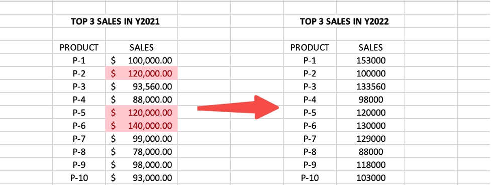
Example: Copy the rule from left side to the right side. The rule is formatting the top 3 values.
Copy the Conditional Formatting Rules by Excel Format Painter Tool
Excel Format Painter allows you to quickly copy the formatting of a cell, range of cells, and apply it to another cell or range. It’s a time-saving feature that helps you maintain consistency in your worksheets.
Here are the steps:
Step1: Select the cell or range that contains the conditional formatting you want to copy.
Step2: Click on the “Format Painter” button in the “Home” tab of the ribbon.
Step3: Click on the cell or range where you want to apply the same conditional formatting rules.
Step4: The conditional formatting should now be applied to the new cell or range.
Copy the Conditional Formatting Rules by Excel “Paste Special” Function
Excel’s “Paste Special” feature allows you to copy and paste data in a variety of ways. The “Formatting” option in Paste Special allows you to copy the formatting of a cell (such as font, color, border styles) without copying the data itself. This is useful when you want to quickly apply a particular formatting style to multiple cells.
Here are the steps:
Step1: Select the cell or range that contains the conditional formatting rules you want to copy.
Step2: Right-click on the selection and choose “Copy” or press “Ctrl + C” on your keyboard.
Step3: Select the cell or range where you want to apply the same conditional formatting rules.
Step4: Right-click on the selection and choose “Paste Special” or press “Ctrl + Alt + V” on your keyboard.
Step5: In the “Paste Special” menu, select “Formatting“.
Step6: The conditional formatting rules will be copied to the new location, and any cell values that meet the same conditions will be formatted accordingly.
Copy the Conditional Formatting Rules by “Conditional Formatting” Function – Duplicate Rules
You can copy conditional formatting rules using the “Duplicate Rules” function in Excel Conditional Formatting. “Duplicate Rules” allow you to easily identify and highlight cells by an existing rule in current worksheet or entire workbook. The only thing you need to do is changing the application destination.
Here are the steps:
Step1: Select the cell or range of cells that has the conditional formatting rule that you want to copy.
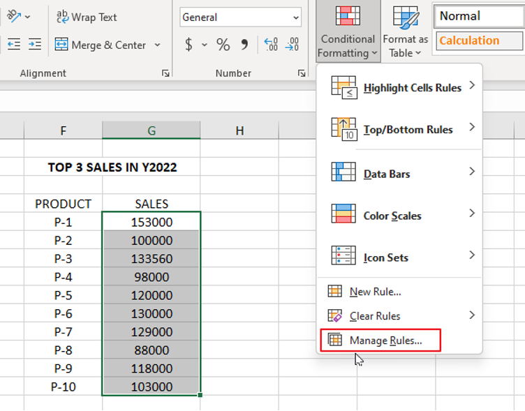
Step2: Click on the “Conditional Formatting” button in the Home tab.
Step3: Select “Manage Rules” from the dropdown menu.
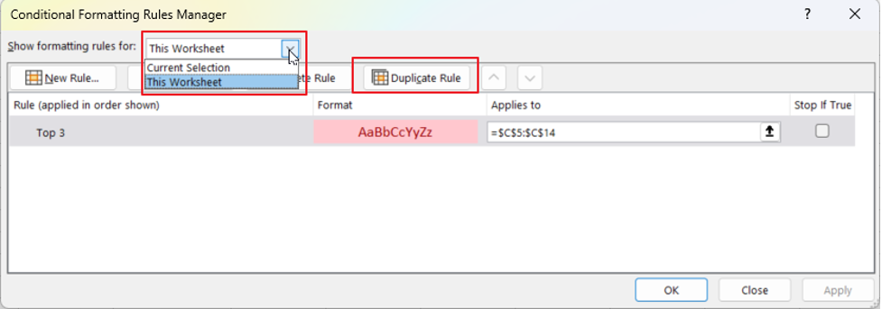
Step4: In the “Conditional Formatting Rules Manager” dialog box, select “This Worksheet” in “Show formatting rules for” dropdown list, select the rule that you want to duplicate, in this example there is only one rule “Top 3”, click on the “Duplicate Rule” button.
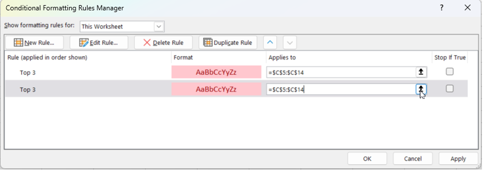
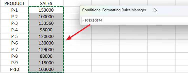
Step5: Two “Top 3” rules are listed in Rule. Select one rule of “Top 3”, click the arrow to modify the “Applies to” to the destination where want to apply the rule.
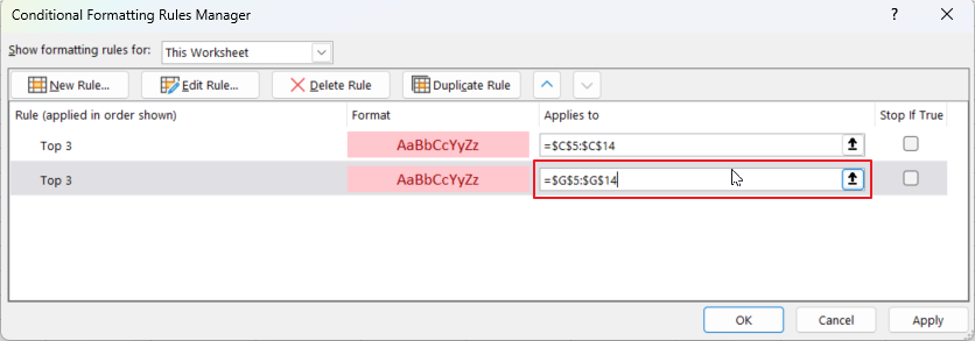
In this example, the destination is G5:G14.
Step6: Click “OK” to apply the rule to the selected range of cells.
Step7: Destination range applied the conditional formatting rule.

Conclusion
The three ways mentioned above are useful when you want to quickly apply a particular formatting style from one range to multiple ranges, without having to manually apply the rule one by one. All three methods can save time and help you become more efficient in your spreadsheet work.