This post will introduce you to the process of inserting worksheets from another workbook in Microsoft Excel using the “Move or Copy” feature. This is a useful method when you need to consolidate data from multiple workbooks into a single workbook, or if you want to reuse existing worksheets across different workbooks.
If you want to insert worksheets from another workbook in Microsoft Excel, just follow these steps:
Step1: Open the destination workbook where you want to insert the worksheets.
Step2: Click on the “Home” tab in the ribbon at the top of the Excel window.
Step3: Click on the “Insert” dropdown in the Cells group, and select “Insert Sheet“.
Step4: Click on the “File” tab in the ribbon at the top of the Excel window, Click on “Open” and navigate to the source workbook. And select the source workbook and click on “Open“.
Step5: In the source workbook, select the worksheet(s) that you want to insert. Right-click on the selected worksheet(s) and click on “Move or Copy“.
Step6: In the “Move or Copy” dialog box, select the destination workbook from the “To book” dropdown. And select the position where you want to insert the worksheet(s) in the destination workbook.
Step7: Select the “Create a copy” checkbox if you want to create a copy of the worksheet(s) rather than moving them.
Step8: Click “OK” to insert the worksheet(s) into the destination workbook.
Alternatively, you can also drag and drop the selected worksheet(s) from the source workbook to the destination workbook. To do this, open both workbooks side by side, select the worksheet(s) in the source workbook, drag and drop them to the desired location in the destination workbook.
Conclusion
Inserting worksheets from another workbook in Microsoft Excel can be a time-saving technique that helps you manage data efficiently. Whether you’re consolidating data from multiple sources or reusing existing worksheets across different workbooks, the “Move or Copy” feature can simplify the process. By following the steps outlined in this post, you can easily insert worksheets from one workbook into another, and keep your data organized and accessible.
This post will introduce you how to import multiple text files into multiple sheets in Excel. You can quickly and easily import multiple text files into separate sheets within a single workbook using VBA code. Let’s get started with the step-by-step instructions for importing multiple text files using VBA.
Import Multiple Text Files to Multiple Sheets with VBA Code
If you have a large number of text files that you need to import into Excel, it can be a time-consuming task to import them one by one. You can achieve it by using VBA code, just do the following steps:
To import multiple text files into multiple sheets with VBA code in Excel, you can follow these steps:
Step1: Open a new workbook in Excel and press ALT + F11 to open the Visual Basic Editor.
Step2: In the Visual Basic Editor, insert a new module by clicking Insert > Module.
Step3: Copy and paste the following VBA code into the new module:
Sub ImportTextFiles_excelgeek()
    Dim FileNames As Variant
    Dim i As Integer
    FileNames = Application.GetOpenFilename(filefilter:="Text Files (*.txt),*.txt", MultiSelect:=True)
    If Not IsArray(FileNames) Then
        Exit Sub
    End If
    For i = LBound(FileNames) To UBound(FileNames)
        With ActiveWorkbook.Sheets.Add(After:=Sheets(Sheets.Count))
            .Name = Left(Right(FileNames(i), Len(FileNames(i)) - InStrRev(FileNames(i), "\")), Len(Right(FileNames(i), Len(FileNames(i)) - InStrRev(FileNames(i), "\"))) - 4)
            .QueryTables.Add Connection:="TEXT;" & FileNames(i), Destination:=.Range("A1")
            .QueryTables(1).TextFilePlatform = xlWindows
            .QueryTables(1).TextFileStartRow = 1
            .QueryTables(1).TextFileParseType = xlDelimited
            .QueryTables(1).TextFileTextQualifier = xlTextQualifierDoubleQuote
            .QueryTables(1).TextFileConsecutiveDelimiter = False
            .QueryTables(1).TextFileTabDelimiter = True
            .QueryTables(1).TextFileSemicolonDelimiter = False
            .QueryTables(1).TextFileCommaDelimiter = False
            .QueryTables(1).TextFileSpaceDelimiter = False
            .QueryTables(1).TextFileOtherDelimiter = ""
            .QueryTables(1).Refresh BackgroundQuery:=False
        End With
    Next i
End Sub
This post will introduce three methods for importing multiple CSV files into one Excel workbook.
The first method involves using VBA code to automate the process of importing CSV files.
The second method involves using Power Query, a data connection technology that allows you to connect to and import data from various sources.
This third method can be used to easily combine multiple CSV files into one Excel worksheet using the command prompt.
Those methods can save time and effort when working with multiple CSV files in Excel.
Import or Merge Multiple CSV Files into Separate Worksheet Using VBA Code
If you try to import or merge multiple CSV files manually into separate worksheets, it should be time-consuming and tedious. You can use VBA code to automate the process to save your time and effort.
To import or merge multiple CSV files into separate worksheets using VBA code, just follow the steps below:
Step1: Open the Excel workbook where you want to import or merge the CSV files.
Step2: Press Alt+F11 to open the Visual Basic Editor.
Step3: In the Visual Basic Editor, select Insert > Module to create a new module.
Step4: Copy and paste the below VBA code into the new module.
Sub ImportCSVFiles_excelgeek ()
    Dim FolderPath As String, Filename As String
    Dim Sheet As Worksheet, NextRow As Long
    Dim FilePicker As FileDialog

    ' Show the File Picker dialog box to select the folder containing the CSV files
    Set FilePicker = Application.FileDialog(msoFileDialogFolderPicker)
    FilePicker.AllowMultiSelect = False
    FilePicker.Title = "Select the folder containing the CSV files"
    If FilePicker.Show <> -1 Then Exit Sub
        FolderPath = FilePicker.SelectedItems(1)
        ' Loop through all CSV files in the folder
        Filename = Dir(FolderPath & "\*.csv")
        Do While Filename <> ""
            ' Open the CSV file
            Workbooks.Open Filename:=FolderPath & "\" & Filename, ReadOnly:=True
            ' Copy the data to a new worksheet
            Set Sheet = ThisWorkbook.Worksheets.Add(After:= _
                  ThisWorkbook.Worksheets(ThisWorkbook.Worksheets.Count))
            Sheet.Name = Left(Filename, Len(Filename) - 4)
            Range("A1").Select
            Selection.CurrentRegion.Select
            Selection.Copy Sheet.Range("A1")
            Workbooks(Filename).Close
            ' Move to the next row on the new worksheet
            NextRow = Sheet.Cells(Rows.Count, 1).End(xlUp).Row + 1
            ' Set the filename to the next file in the folder
            Filename = Dir
        Loop
End Sub
Step5: Save the module and return to the Excel workbook.
Step6: Press Alt+F8 to open the Macro dialog box, or click on the Macros command under Code group and select the macro you just created. Click Run to execute the macro.
Step7: You need to select one folder that containing the CSV files.
Step8: The macro will automatically import or merge the CSV files into separate worksheets in the same workbook.
This code will display the File Picker dialog box to select the folder containing the CSV files. It will then loop through all CSV files in the folder, open each file, and copy the data into a new worksheet in the same workbook. The name of each worksheet will match the name of the CSV file, without the “.csv” extension.
Note: Before running the macro, make sure the CSV files are located in the same folder. Also, if you have a large number of CSV files to import or merge, it may take some time to complete the process.
Import or Merge Multiple CSV Files into one Excel Worksheet using Command Prompt
If you want to import or merge multiple CSV files into one Excel worksheet, and you can achieve it by using the command prompt in Windows command line, just do the following steps:
Step1: Open the Command Prompt. On Windows, you can press the Windows key + R, type “cmd“, and press Enter.
Step2: Navigate to the folder where your CSV files are located using the “cd” command.
Step3: Type “copy *.csv mergedfiles.csv” command and press Enter.
This will create a new file named “ mergedfiles.csv ” that contains the data from all the CSV files in the folder.
Step4: Open Microsoft Excel and select “Open” from the “File” menu.
Step5: In the “Open” dialog box, navigate to the folder where your CSV files are located. And Change the file type to “All Files“. Select the “ mergedfiles.csv ” file and click “Open“.
Step6: In the Text Import Wizard, select “Delimited” as the file type and click “Next“.
Step7: Select “Comma” as the delimiter and click “Next“.
Step8: click on “Finish” command, the csv file would be imported into the current worksheet.
Import or Merge Multiple CSV Files into one Excel Worksheet using Power Query
You can import or merge multiple CSV files into one Excel worksheet using Power Query, just do the following steps:
Step1: Open Microsoft Excel and select “Data” Tab.
Step2: Click on “From File” in the “Get & Transform Data” section. And Select “From Folder” in the drop-down menu.
Step3: In the “FromFolder” dialog box, navigate to the folder where your CSV files are located and click “Open“. The Power Query window will open.
Step4: select “Combine & Transform Data” from the Power Query window. And the Combine Files window will appear.
Step5: In the “Combine Files” dialog box, choose the Delimiter option as Comma based on your csv data and click “OK“.
Step6: In the Power Query Editor dialog box, select the columns you want to include in the merged table. You can now edit, filter, and transform the merged data as needed.
Step7: Click “Close & Load” to import the merged data into Excel.
Step8: This will merge the data from all the CSV files in the selected folder into one table in Excel using Power Query.
Note: if the CSV files have different structures, the merged table may not import correctly.
Conclusion
There are several ways to import or merge multiple CSV files into one Excel workbook. VBA code can be used to merge the files into one workbook, while using command prompt can be a quick and simple solution for those who prefer a command-line interface. On the other hand, using Power Query is a more user-friendly solution that allows for editing, filtering, and transforming the data, and can be particularly useful for large datasets.
This post will introduce you to the concept of QueryTables in Excel VBA. QueryTables is an object that allow you to import data from external sources, such as databases, web pages, and text files, directly into your Excel workbook.
In this post, we will discuss how to create, refresh, and delete QueryTables using VBA code, and we’ll provide examples of how to use QueryTables with different types of data sources.
Creating a New QueryTable
If you want to create a new QueryTable, you can use the Add method of the QueryTables collection of a Worksheet object.
The Add method has several parameters that you can use to customize the QueryTable, such as the Connection parameter, which specifies the data source, and the Destinationparameter, which specifies the range of cells where the data should be imported.
Here’s an example of how to create a new QueryTable in VBA:
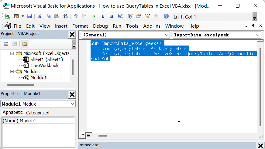
Sub ImportData_excelgeek()
    Dim myquerytable  As QueryTable
    Set myquerytable = ActiveSheet.QueryTables.Add(Connection:="ODBC;DSN=DatabaseName;UID=Username;PWD=Password", Destination:=Range("A1"))
End Sub
In this example, the Connection parameter specifies an ODBC connection to a database, and the Destination parameter specifies that the imported data should be placed in cell A1 of the current worksheet.
Specifying Data Source
The Connection parameter is used to specify the data source for the QueryTable. The syntax of the Connection parameter depends on the type of data source you are using.
If you want to import data from a web page, you can use the following connection parameter:
In this example, the ODBC connection uses the Data Source Name (DSN) ” DatabaseName “, the username ” Username “, and the password ” Password “.
Refreshing the QueryTable
Once you have created a QueryTable, you can refresh it by calling the Refreshmethod of the QueryTable object.
Here’s an example of how to refresh a QueryTable:
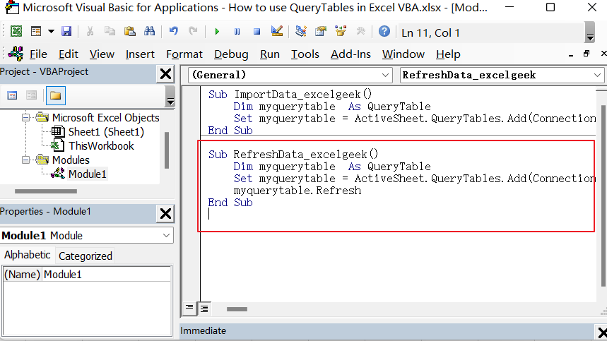
Sub RefreshData_excelgeek()
    Dim myquerytable  As QueryTable
    Set myquerytable = ActiveSheet.QueryTables.Add(Connection:="ODBC;DSN=DatabaseName;UID=Username;PWD=Password", Destination:=Range("A1"))
    myquerytable.Refresh
End Sub
In this example, the RefreshData_excelgeek subroutine gets a reference to the first QueryTable in the active sheet’s QueryTables collection, and then calls the Refreshmethod of the QueryTable to refresh the data.
Cleaning up QueryTable
After you have finished using a QueryTable, you should clean it up by calling the Deletemethod of the QueryTable object.
Here’s an example of how to delete a QueryTable:
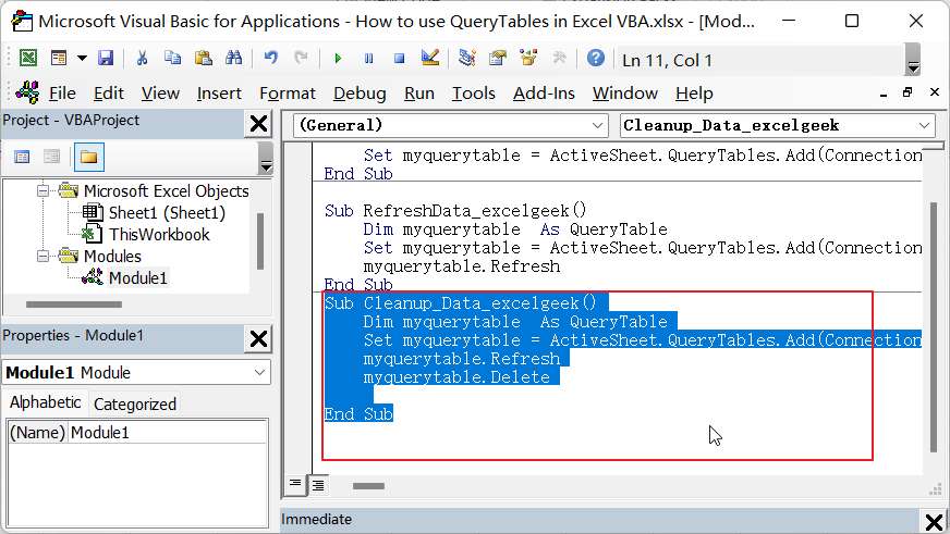
Sub Cleanup_Data_excelgeek()
    Dim myquerytable  As QueryTable
    Set myquerytable = ActiveSheet.QueryTables.Add(Connection:="ODBC;DSN=DatabaseName;UID=Username;PWD=Password", Destination:=Range("A1"))
    myquerytable.Refresh
    myquerytable.Delete
End Sub
In this example, the Cleanup_Data_excelgeek subroutine gets a reference to the first QueryTable in the active sheet’s QueryTables collection, and then calls the Deletemethod of the QueryTable to delete it.
This post will introduce you to the process of importing a text file or CSV (Comma Separated Values) file into Excel. If you’re working with a large dataset, importing the data into Excel can save you time and effort compared to manually entering the data.
Excel provides several tools and methods for importing data from external sources, including text files and CSV files. In this article, we’ll show you how to use these tools and provide step-by-step instructions for importing a text file or CSV file into Excel.
Import Text File or CSV File into Excel Using From Text/CSV Feature
Here are the detailed step-by-step instructions for importing a text file or CSV file into Excel:
Step1: Open a new or existing Excel workbook.
Step2: Go to the “Data” tab on the ribbon and click on “From Text/CSV” in the “Get & Transform Data” group. If you’re using an older version of Excel, you may need to go to the “Data” tab and click on “From Text” instead.
Step3: Navigate to the location of the text or CSV file you want to import and select it. If the file is not in the default location, you can click on the “Browse” button to search for it. then click on the Import button.
Step4: The Text Import Wizard will open in the Microsoft Excel Spreadsheet. Choose one delimiter based on your imported file, such as: Tab character.
Step5: Once you’re satisfied with the settings, click on the “Load” button to import the data into Excel. The data will be inserted into a new worksheet in the workbook.
Note: this method is only available on Excel 2016, Excel 2019, Excel 365 or higher versions.
Open Text File Using with Open Command in Excel
You can also use the “Open” command to open or import a text file or CSV file. Here are the steps:
Step1: Open a new or existing Excel workbook.
Step2: Go to the “File” tab on the ribbon and click on “Open“.
Step3: Navigate to the location of the text or CSV file you want to import and select it.
Step4: In the “Open” dialog box, select “Text Files” or “All Files” from the drop-down menu next to “File name”. If you don’t see the file type you want to import, you can select “All Files” and then locate the file manually.
Step5: Select the file you want to import and click on “Open“.
Step6: The Text Import Wizard will open. The first step is to select the file type. By default, Excel will detect the file type based on the file extension, but you can also select the file type manually. For a text file or CSV file, you should select “Delimited“. Click Next button.
Note: You can also specify other settings in the Text Import Wizard. For example, if the file contains headers (column names), you can select the “My data has headers” option.
Step7: you need to specify the delimiter used in the file. Choose Tab checkbox as delimiters. Click Next button.
Note: A delimiter is a character that separates the values in each column. The most common delimiter is a comma (,), but you can also use a tab character (\t) or a semicolon (;), depending on the file.
Step8: Preview the data to make sure it looks correct in Data Preview section. If you need to make any changes, you can go back to the previous steps in the Text Import Wizard. Click “Finish” button.
Step9: Click on the “Load” button to import the data into Excel. The data will be inserted into a new worksheet in the workbook.
If you want to import multiple text files, and you can go back to the “From Text/CSV” dialog box and repeat the above steps for each file.
Import CSV File to Worksheet with VBA Code
You can also import CSV file to a worksheet with VBA code in Excel, and you just need a few lines of VBA code, and you can quickly import a CSV file into a new worksheet in the active workbook.
Just do the following steps:
Step1: Press Alt + F11 to open the Microsoft VBA editor
Step2: From the menu bar, choose Insert > Module
Step3: In the Module window, paste the following VBA code.
Sub ImportCSV()

    ' Prompt the user for the path and filename of the CSV file
    Dim filePath As String
    filePath = Application.GetOpenFilename("CSV File (*.csv), *.csv", , "excelgeek for Excel", , False)
    ' Check if the user canceled the input box
    If filePath = "" Then
        MsgBox "No file selected. Import canceled.", vbExclamation, "Import CSV"
        Exit Sub
    End If

    Set rangeAddress = Application.InputBox("please select a cell to output csv data", "excelgeek for Excel", Application.ActiveCell.Address, , , , , 8)

    ' Import the CSV file into a new worksheet in the active workbook
    With ActiveSheet.QueryTables.Add(Connection:="TEXT;" & filePath, Destination:=Range(rangeAddress.Address))
        .TextFileParseType = xlDelimited
        .TextFileCommaDelimiter = True
        .Refresh
    End With
End Sub
Note: This code uses the QueryTables.Addmethod to import the CSV file into a new worksheet in the active workbook. You can specify the file path, delimiter, and destination for the imported data.
Step4: Press F5 to run the code, or press the “Run” button on the toolbar
Step5: You need to select one CSV file in the Import dialog box.
Step6: you need to select one cell to output the csv data that you want to import.
Step7: The selected CSV data will be inserted into the current worksheet.
Conclusion
Importing text files or CSV files into Excel is very useful and it can save you time and effort when working with large datasets. With the built-in tools and methods provided by Excel, you can easily import your data and begin analyzing, manipulating, and visualizing it in a meaningful way.
This post will introduce the DAVERAGE function in Excel and provide a step-by-step guide on how to use it. The DAVERAGE function can be used to calculate an average value based on criteria in a database or table.
This function can be particularly useful when dealing with large amounts of data, as it allows you to calculate the average for specific subsets of the data.
In this post, we will cover the basics of the DAVERAGE function and provide examples of how you can use it in your own analysis.
How To Use DAVERAGE Function
The DAVERAGE function in Excel is a powerful tool for calculating the average of a set of values in a database or table based on specific criteria.
The Syntax of the DAVERAGE function is as below:
=DAVERAGE(database, field, criteria)
The CUBEVALUE function takes the following arguments:
connection: A string that specifies the OLAP database connection.
expression: A string that specifies the measure or calculated member to retrieve.
member1, member2, …: Optional strings that specify the members to filter the data.
The DAVERAGE Function Example
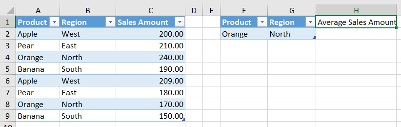
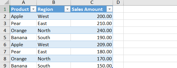
Assuming that you have a large dataset or data table for a company, and you want to calculate the average sale amount for a specific product (Orange) in a specific region (North). You can use the below DAVERAGE function to achieve it.
Just do the following steps:
Step1: Modify your data range(A1:C10) is in a tabular format with headers.
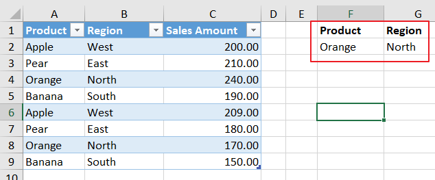
Step2: You need to setup a criteria range in Cells F1:G2, with “Product” in Cell F1 and “Region” in Cell G1, and “Orange” and “North” in Cells F2 and G2.
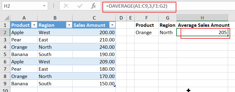
Step3: select a cell where you want to display the result of the DAVERAGE function. For example, select Cell H2 and type the below DAVERAGE formula, then press Enter key to calculate the final result.
=DAVERAGE(A1:C9,3,F1:G2)
Conclusion
You can use the DAVERAGE function to easily perform complex calculations on large datasets in Excel, and obtain specific results based on the criteria you set.
This post will introduce the CUBEVALUE function in Excel and provide a step-by-step guide on how to use it. The CUBEVALUE function is a powerful tool that allows users to retrieve data from a cube in an OLAP (Online Analytical Processing) database.
In this post, we’ll cover the basics of the CUBEVALUE function and provide examples of how you can use it in your own analysis.
How To Use CUBEVALUE Function
The CUBEVALUE function in Excel is a powerful tool for retrieving data from a cube in an OLAP database.
The CUBEVALUE function takes the following arguments:
connection: A string that specifies the OLAP database connection.
expression: A string that specifies the measure or calculated member to retrieve.
member1, member2, …: Optional strings that specify the members to filter the data.
If you want to use the CUBEVALUE function with a data model, you must first create a connection to the OLAP database that contains the data model. Once you have created the connection, you can use the CUBEVALUE function to retrieve data from the data model.
The CUBEVALUE function Example
Here are some examples of how to use the CUBESET function in Excel:
Example1:
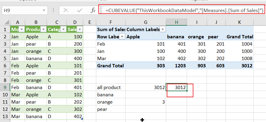
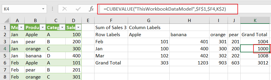
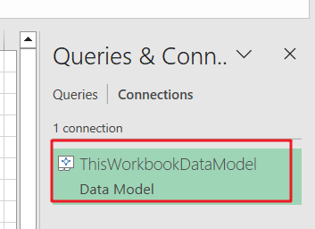
Suppose you have a cube data source named “ThisWorkbookDataModel” and you want to retrieve the total sales for all products in the data set, and you can use the following formula:
=CUBEVALUE("ThisWorkbookDataModel","[Measures].[Sum of Sales]")
Example2:
If you want to retrieve the total sales for all products in the Jan, you can use the following CUBEVALUE function:
=CUBEVALUE("ThisWorkbookDataModel",$F$1,$F4,K$2)
Where,
F1 =CUBEMEMBER(“ThisWorkbookDataModel”,”[Measures].[Sum of Sales 3]”)
You can use Excel CUBEVALUE function to create dynamic reports and analysis that can help you gain insights into your data. Whether you’re working with financial data, sales data, or any other type of data, the CUBEVALUE function can be a valuable tool in your analysis toolkit.
This post will introduce a method to copy data from one Microsoft Excel workbook to another using Visual Basic for Applications (VBA) code, without having to open the source workbook. This process can save time and effort when working with large amounts of data and can help automate tedious manual processes.
By utilizing VBA in Excel, it is possible to copy data from another workbook without opening it, allowing for a streamlined and efficient data transfer process.
What is EXCEL VBA?
Excel VBA (Visual Basic for Applications) is a programming language that allows users to automate tasks and create custom functionality in Microsoft Excel. VBA enables users to write macros, scripts, and programs that can perform various actions within Excel, such as copying and pasting data, formatting cells, generating reports, and much more.
By using VBA, Excel users can create custom solutions that can save time and increase productivity by automating repetitive tasks. VBA provides a simple and easy-to-use interface for users to interact with Excel, allowing them to create custom functions, forms, and dialog boxes to enhance the functionality of the software.
Copy Data from a Closed Workbook with VBA in Excel
You can copy data from another workbook without opening it using VBA in Microsoft Excel.
By using VBA, it is possible to automate the process of copying data from one workbook to another, saving time and effort. The process involves using the Workbooks.Open method to open the source workbook in memory, selecting the range of data to be copied, and then using the PasteSpecial method to paste the data into the target workbook. Here’s an example code that demonstrates this process:
Sub CopyDataWithoutOpening()
    Dim sourceFilePath As String
    Dim targetFilePath As String

    sourceFilePath = "D:\sourcesheet.xlsx"
    targetFilePath = "D:\targetsheet.xlsx"

    With Workbooks.Open(sourceFilePath)
        .Sheets("Sheet1").Range("A1:C5").Copy
    End With     Workbooks.Open(targetFilePath).Sheets("Sheet1").Range("A1").PasteSpecial xlPasteValues
End Sub
This code assumes that both the source and target workbooks have a sheet named “Sheet1“, and that the data you want to copy is in the range ” A1:C5” in the source workbook. Replace sourceFile and targetFile with the actual file paths of the source and target workbooks, respectively.
Apply VBA Code to Copy Data From one workbook to another closed workbook
To apply the above VBA code to copy data from one workbook to another without opening the source workbook in Microsoft Excel, follow these steps:
Step1: Open the target workbook in Microsoft Excel
Step2: Press Alt + F11 to open the Microsoft VBA editor
Step3: From the menu bar, choose Insert > Module
Step4: In the Module window, paste the code
Step5: Update the values of sourceFilePath and targetFilePath variables to the actual file paths of the source and target workbooks, respectively
Step6: Press F5 to run the code, or press the “Run” button on the toolbar
Step7: The data from the source workbook should now be copied to the target workbook, without opening the source workbook.
Note: Make sure that the source workbook is not open when you run this code, or you will receive an error message.
This post will explain the process of creating a Data Model in Excel. We will cover the steps involved in creating a Data Model, from importing data to creating relationships between tables. By the end of this post, you will have a solid understanding of how to use the Data Model in Excel and harness its full potential.
What is Data Model?
A data model in Excel is a representation of data that provides a structure for organizing and analyzing large amounts of data. It allows you to import data from multiple tables and create relationships between the tables, so that you can easily combine and analyze the data in new ways.
The Data Model in Excel is stored in a compact and efficient format that is optimized for fast data analysis, and it supports powerful features such as pivot tables, pivot charts, and DAX formulas. By using the Data Model in Excel, you can simplify the process of working with large data sets, and perform complex data analysis tasks with ease.
Create Data Model in Excel
If you want to create a data model in Excel, you can follow these steps:
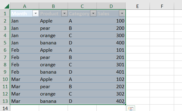
Step 1: You need to Convert your data into tables with unique headers and select this table.
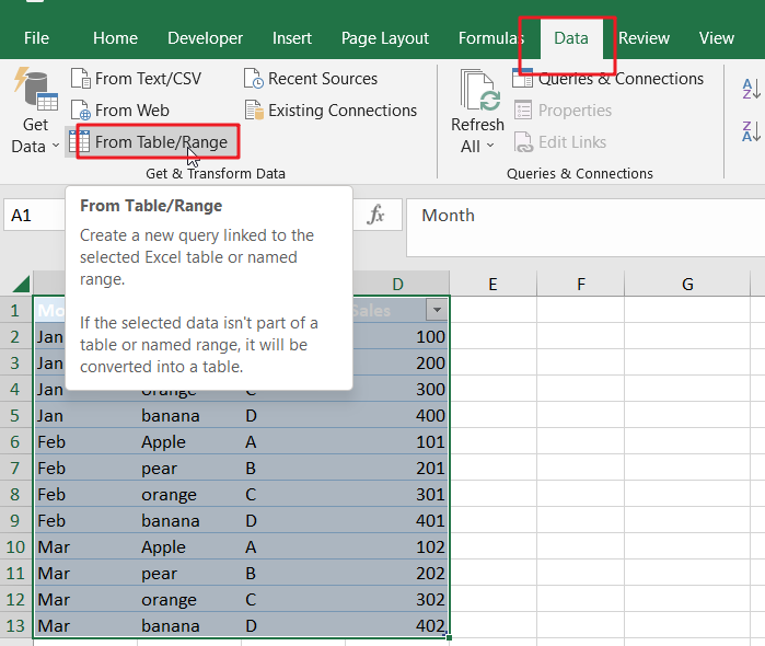
Step 2: then you need to go to the “Data” tab and click “From Table/Range“.
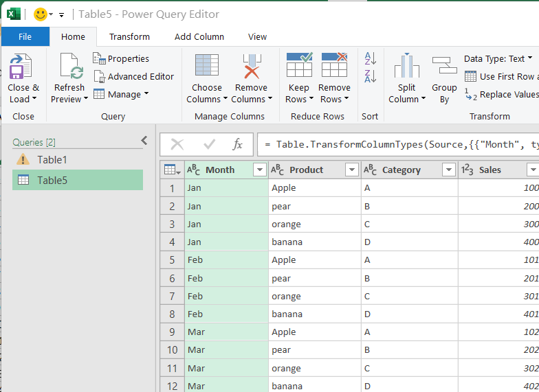
Step 3: Select the current table you want to include in the data model in the Power Query Editor window and click “Close &Load“.
Step 4: Repeat the process for any additional tables you want to include in the data model.
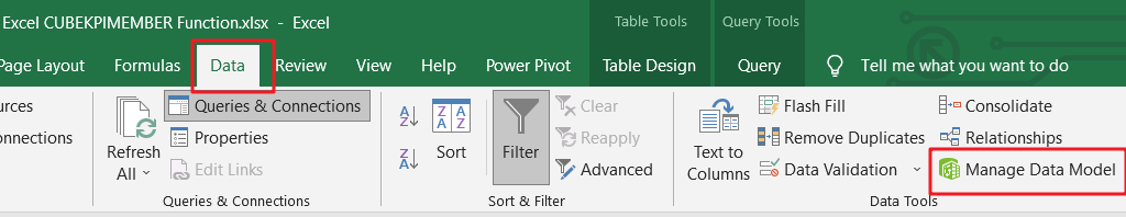
Step 5: then click the “Manage Data Model” button in the “Data Tools” group.
Step 5: You can now use the data model to create pivot tables, pivot charts, and other data visualizations that summarize and analyze your data.
Note: The steps assume that you are using Microsoft Excel 2016 or later. The process may differ slightly in earlier versions of Excel.
Data Model Examples in Microsoft Excel Spreadsheet
The above steps have been created one data model named as “ThisWorkbookDataModel”. This Section will show you how to add a key performance indicator (KPI) to your data model(ThisWorkbookDataModel) in Excel.
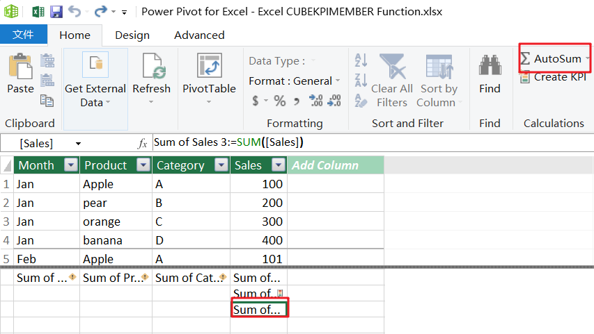
Step 1: You can click the “Manage Data Model” button in the “Data Tools” group.
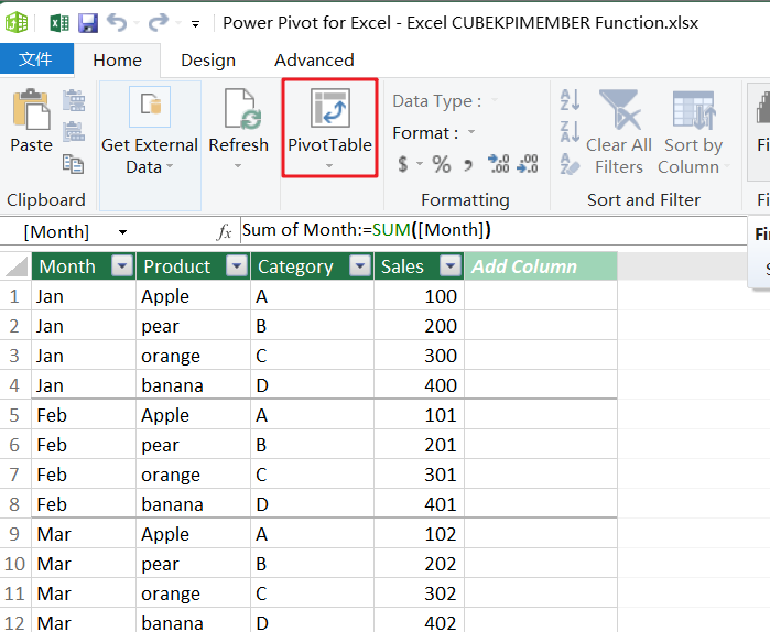
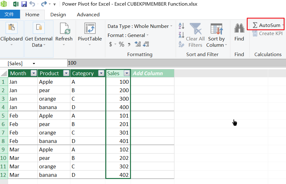
Step 2: select Sales column, and then click on AutoSum button, and the Sum of Sales measure would be created.
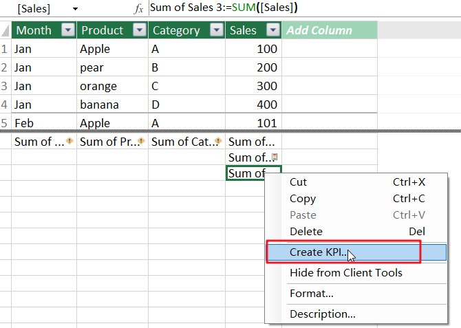
Step 3: right click on the Sum of Sales measure and then select Create KPI.
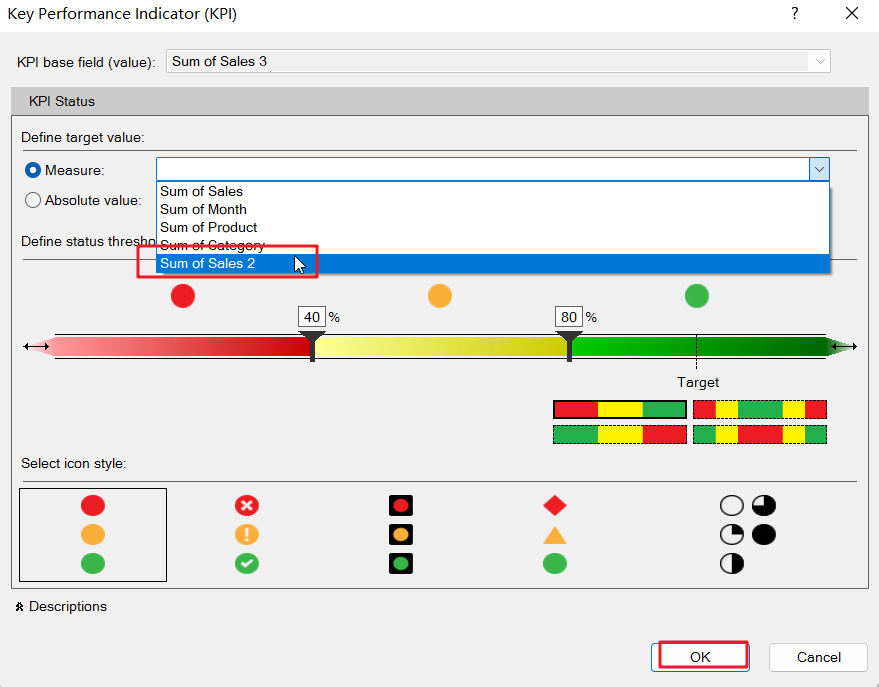
Step 4: The Key Performance Indicator dialog box will open. And choose the Sum of Sales Measure from the drop down list, and click on Ok button.
This post will introduce the Excel CUBESETCOUNT function. The CUBESETCOUNT function is used to count the number of items in a set retrieved from a cube data source in Microsoft Excel Spreadsheet. It is an important tool for data analysis and helps you to understand the size of your data sets and the relationships between them.
Whether you are working with a large data set or a small one, the CUBESETCOUNT function will allow you to efficiently count the items in your sets and make informed decisions based on your data.
The Excel CUBESETCOUNT function is only available in Microsoft Excel 2010 and later versions that support PivotTable reports and cube data source connections. It is not available in earlier versions of Excel or in other spreadsheet applications.
If you are using an earlier version of Excel or a different spreadsheet application, you will not be able to use the CUBESETCOUNT function and will need to use alternative methods for counting the items in your sets.
How To Use CUBESETCOUNT Function
The CUBESETCOUNT function in Excel is used to count the number of items in a set that is retrieved from a cube data source.
The syntax for the CUBESETCOUNT function is as follows:
=CUBESETCOUNT(cube_name, set_expression)
Where:
“cube_name” is the name of the cube data source that you want to retrieve data from.
“set_expression” is the expression that defines the set of items that you want to count.
The CUBESETCOUNT function Example
Here is an example of how to use the CUBESET function in Excel:
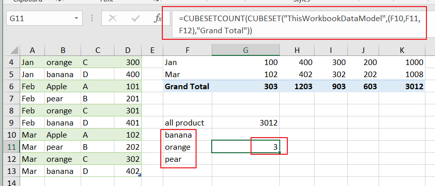
Suppose you have a cube data source named “ThisWorkbookDataModel” and you want to count the number of items in a set . To do this, you would use the following formula:
This formula would return the number of items in the set that represents the product.
When should you not use CUBESETCOUNT in Excel?
The CUBESETCOUNT function is used to count the number of items in a set created from a multi-dimensional data source, such as an OLAP cube. It is important to note that the CUBESETCOUNT function only works with data that is organized in an OLAP cube.
Therefore, if you are not working with data that is organized in an OLAP cube, you should not use the CUBESETCOUNT function as it will not produce meaningful results. Instead, you should use a different function that is more appropriate for your data, such as COUNT, COUNTIF, or SUMIF, depending on your needs.
What are the formulas similar to CUBESETCOUNT in Excel?
Here are some similar formula to CUBESETCOUNT in Excel:
CUBEKPIMEMBER: Returns the unique name of a Key Performance Indicator (KPI) in the cube hierarchy.
CUBEMEMBERPROPERTY: Returns the value of a property for a specified member in the cube hierarchy.
CUBERANKEDMEMBER: Returns the nth, or ranked, member in a set, based on a specified measure.
CUBEVALUE: Returns a value from a cube, based on a specified set of members.
Conclusion
CUBESETCOUNT function in Excel is a powerful tool for aggregating data from a cube or data model. It allows users to count the number of items in a set, which can be useful in a variety of applications, from financial modeling to data analysis.