Copying a cell with a single click can save time and effort compared to using the traditional copy and paste method. This is particularly useful if you frequently need to copy data from a particular cell or range of cells. With the automatic copy feature, you can avoid the risk of accidentally copying the wrong data or overwriting existing data in your worksheet. This post provides a tip on one-click copying in Excel via VBA code.
One-Click Copy by Excel VBA Code
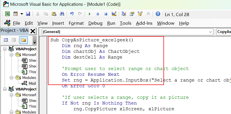
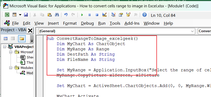
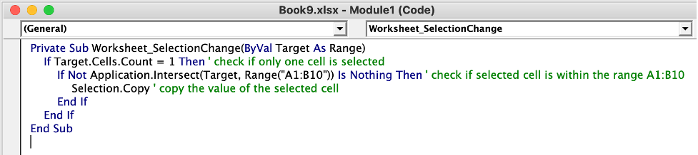
If you are not familiar with the VBA code, you can use the following VBA code to copy the value of a cell to the clipboard with a single click:
Private Sub Worksheet_SelectionChange(ByVal Target As Range)
If Target.Cells.Count = 1 Then
If Not Application.Intersect(Target, Range("A1:B10")) Is Nothing Then
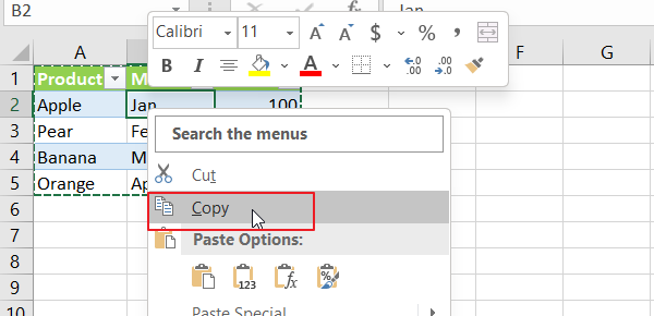
Selection.Copy
End If
End If
End Sub
In this code, “Worksheet_SelectionChange” is a built-in event in Excel VBA that is triggered whenever a cell is selected in the worksheet.
The “If” statement checks if only one cell is selected, so that the code only runs when a single cell is clicked.
The “Application.Intersect” function is used to check if the selected cell is within the specified range (A1:B10 in this example). If the selected cell is within the range, then the value of the selected cell is copied using the “Selection.Copy” method.
Here are the complete steps to use this code in your Excel workbook:
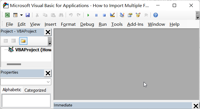
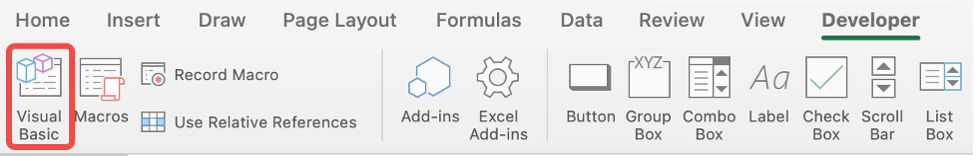
Step1: Press Alt + F11 to open the Visual Basic Editor. Or click the Visual Basic of Developer tab in the ribbon.
Step2: In the Visual Basic Editor window, select the worksheet where you want to enable the copy action.
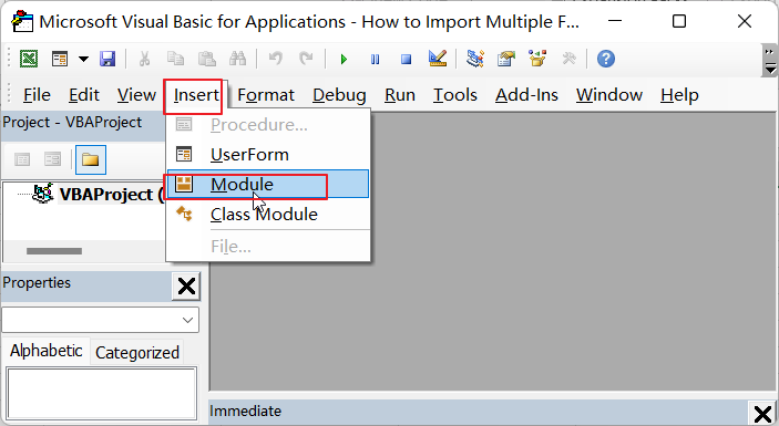
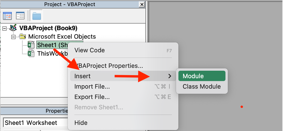
Step3: Right-click the worksheet and insert module by select “Insert” -> “Module” in the menu.
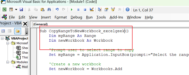
Step4: Copy and paste the code above into the code window.
Step5: Save the workbook and close the Visual Basic Editor.
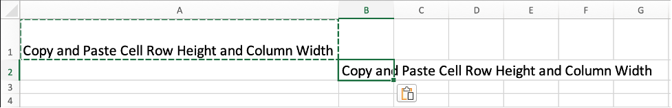
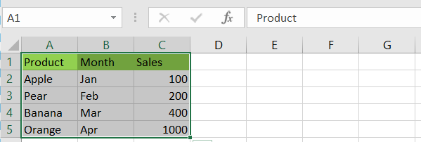
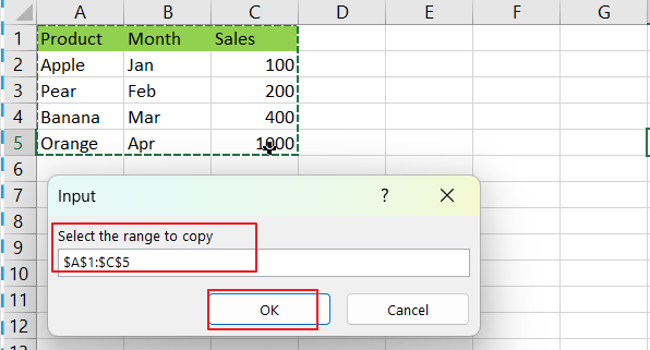
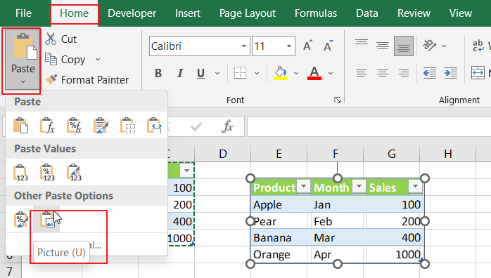
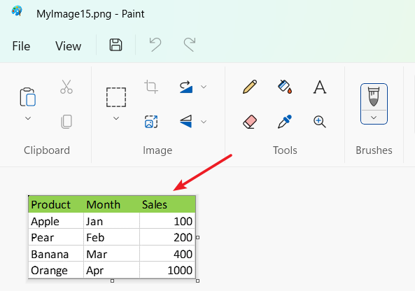
Now, when you click on any cell in the worksheet, its value will be copied to the clipboard automatically. Select a cell where you want to paste the copied cell, press Ctrl+V to paste the content saved in the cell.
If you want to remove the restriction on one cell, you can remove the “if” statement about checking that a cell is selected. You can use the following VBA code to copy a range by single click/select.
Private Sub Worksheet_SelectionChange(ByVal Target As Range)
        If Not Application.Intersect(Target, Range("A1:B10")) Is Nothing Then
            Selection.Copy
        End If
End Sub