Welcome to WordPress. This is your first post. Edit or delete it, then start writing!
Author: will
How to Export Excel Data to Text Files in Excel
This post will explain how to export Excel data to text files in Excel using VBA code. This post will show you how to export one sheet to text files in Excel, which can be useful if you need to extract data from Excel and use it in another program that requires a text file format.
You can easily select the data you want to export, specify a file name and location for the text file, and then generate a text file that contains the data in the format you need.
Export one Single Worksheet to Text File
If you want to export a single Excel sheet to a text file, follow these steps:
Step1: Open the Excel workbook that contains the sheet you want to export.
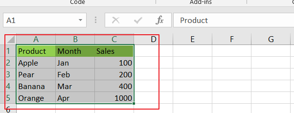
Step2: Click on the sheet you want to export.
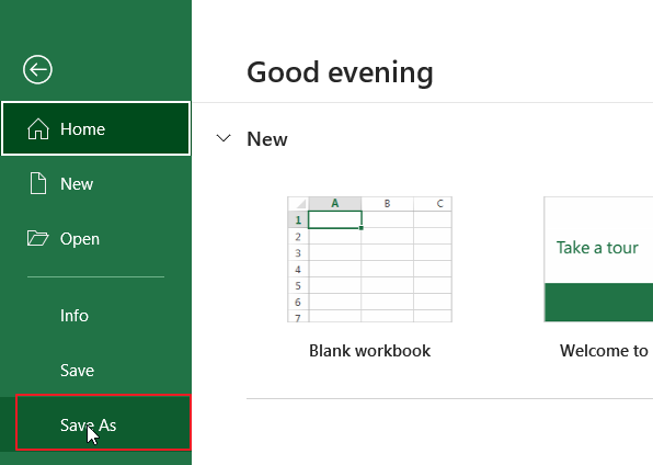
Step3: Click on the “File” tab in the ribbon menu.
Step4: Click on “Save As” in the left-hand menu.
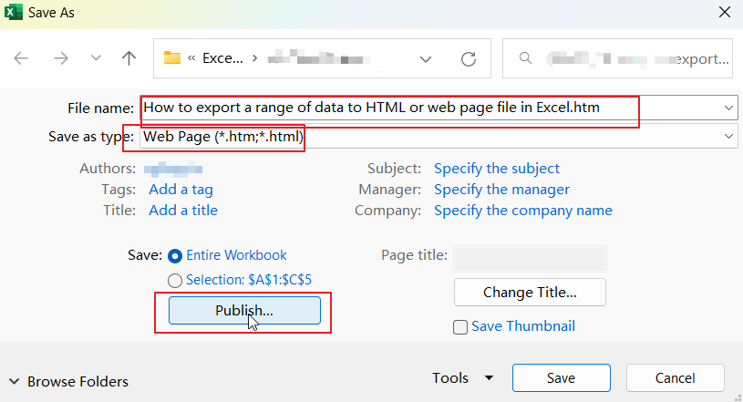
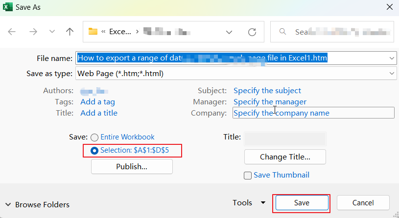
Step5: In the “Save As” dialog box, choose the location where you want to save the text file.
Step6: In the “Save as type” dropdown menu, select “Text (Tab delimited) (*.txt)“.

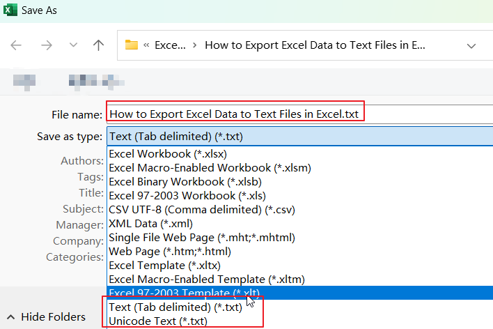
Step7: Click on the “Save” button.
Export one Column or Selection to Text File with VBA Code
You can use VBA code to export a selection or one column to a text file in Excel. Here are the steps:
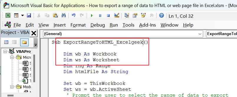
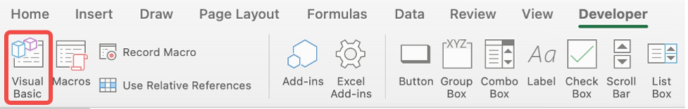
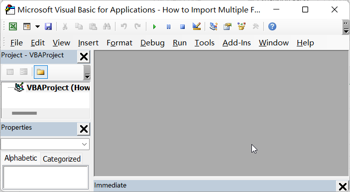
Step1: Press “Alt + F11” on your keyboard. This will open the Visual Basic Editor window.

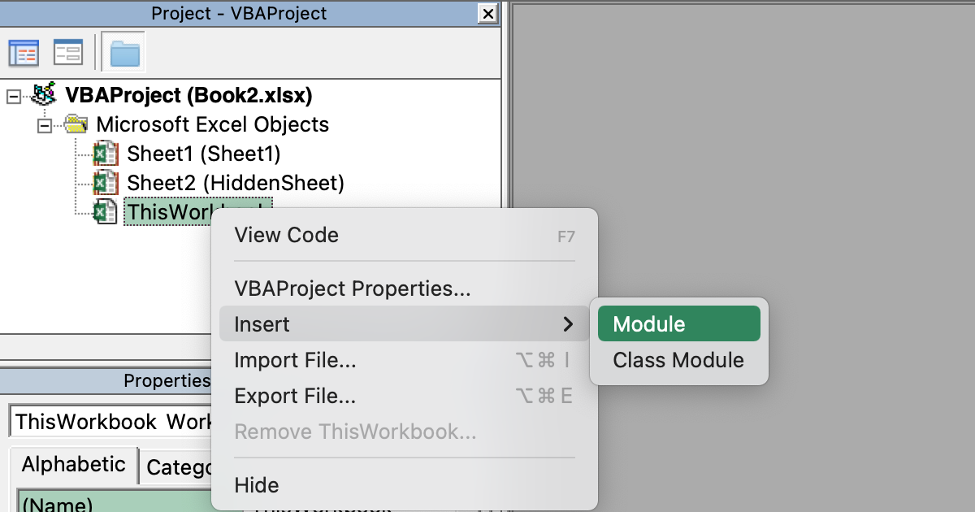
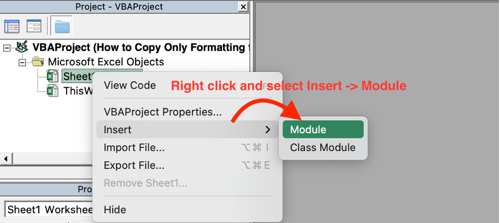
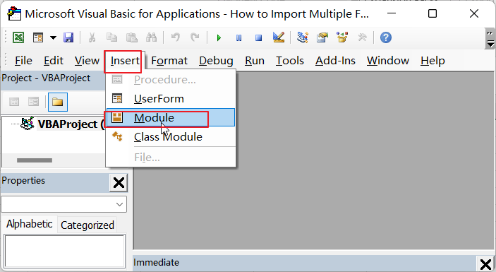
Step2: In the Visual Basic Editor window, select “Insert” from the top menu and choose “Module” to create a new module.
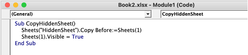
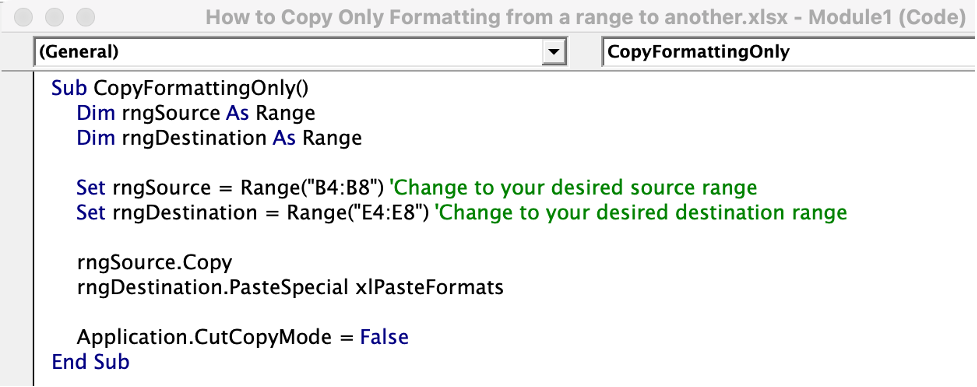
Step3: Copy and paste the following VBA code into the new module. Save the workbook with the VBA code.

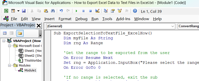
Sub ExportSelectionToTextFile_ExcelHow()
Dim myFile As String
Dim rng As Range
'Get the range to be exported from the user
On Error Resume Next
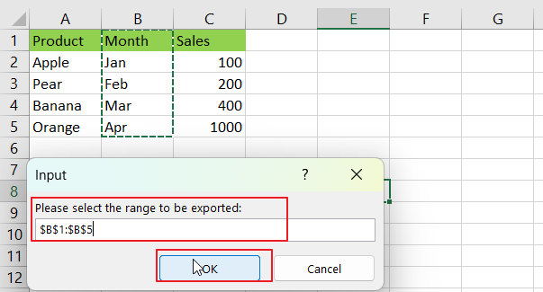
Set rng = Application.InputBox("Please select the range to be exported:", Type:=8)
On Error GoTo 0
'If no range is selected, exit the sub
If rng Is Nothing Then Exit Sub
'Create a new workbook and copy the selected range to it
Dim wb As Workbook
Set wb = Workbooks.Add
rng.Copy Destination:=wb.Sheets(1).Range("A1")
'Get the file name and location for the text file
myFile = Application.GetSaveAsFilename(InitialFileName:="ExportedData.txt", FileFilter:="Text Files (*.txt), *.txt")
'If the user cancels the file selection, exit the sub
If myFile = "False" Then Exit Sub
'If the file name is not valid, display an error message and exit the sub
If Len(myFile) = 0 Then
MsgBox "Invalid file name. Please select a valid file name and location.", vbExclamation, "Export to Text File"
Exit Sub
End If
'Save the new workbook as a text file and close it
wb.SaveAs FileName:=myFile, FileFormat:=xlText, CreateBackup:=False
wb.Close SaveChanges:=False
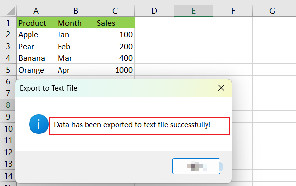
'Display a success message
MsgBox "Data has been exported to text file successfully!", vbInformation, "Export to Text File"
End Sub
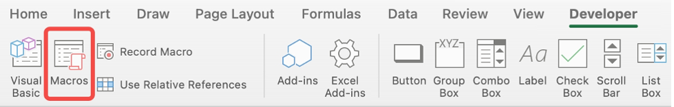
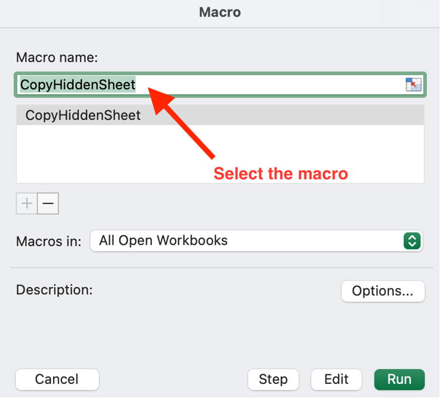
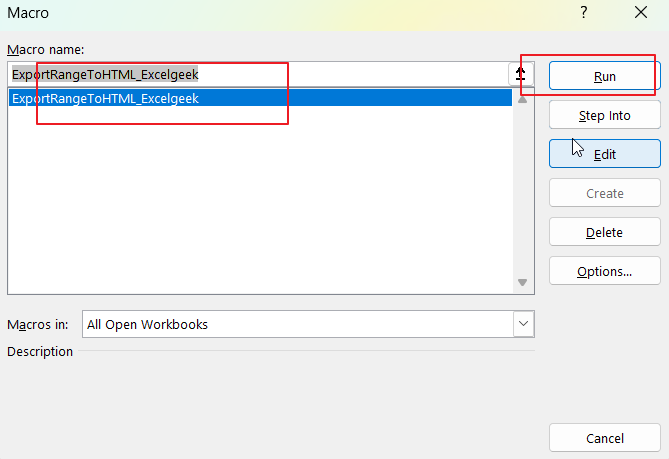
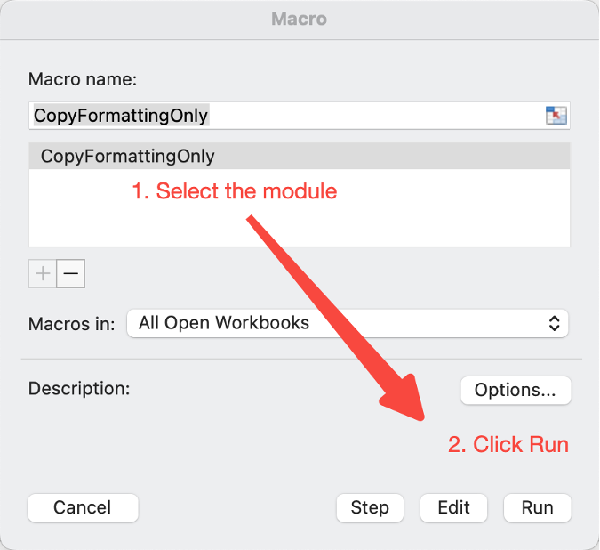
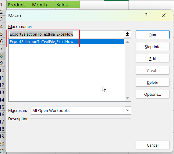
Step4: Press “Alt + F8” to open the Macro dialog box. Select the ” ExportSelectionToTextFile_ExcelHow” macro from the list of macros and click “Run“.

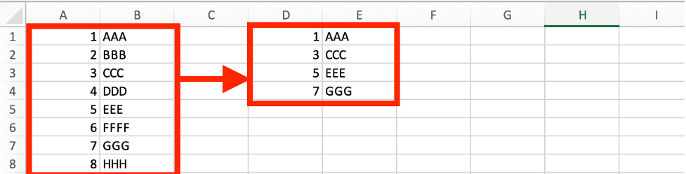
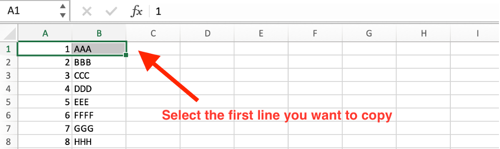
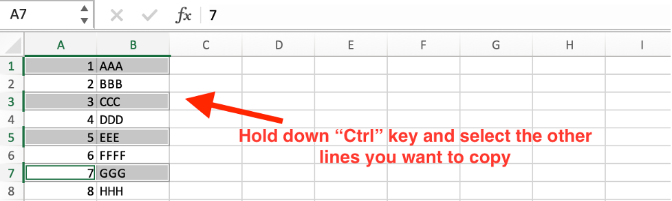
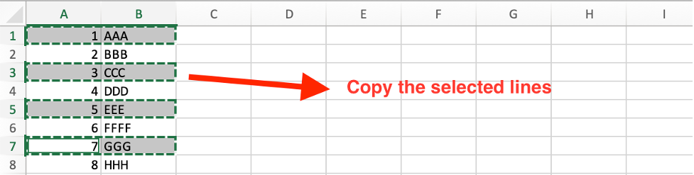
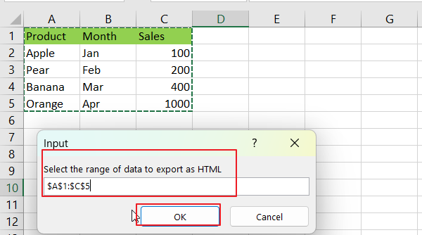
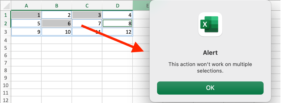
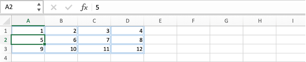
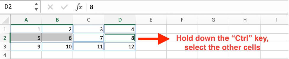
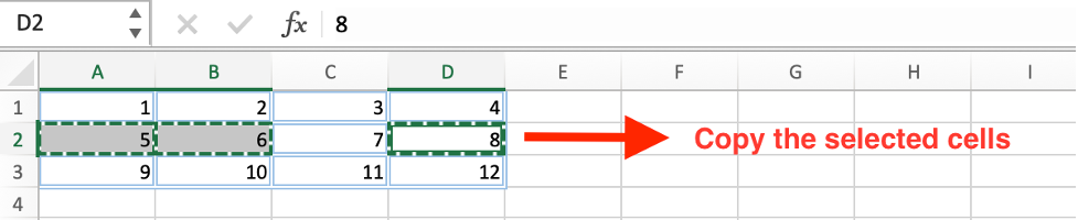
Step5: select the range to be exported

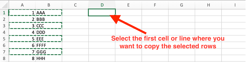
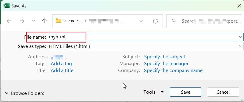
Step6: select a file name and location for the text file to be exported.

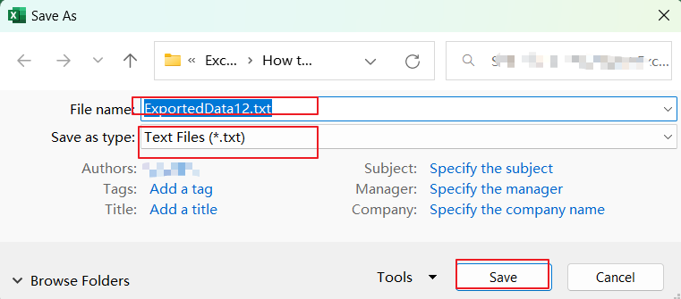
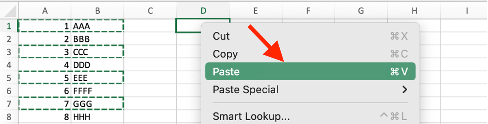
Step6: Click “Save” to export the selected range to the text file.

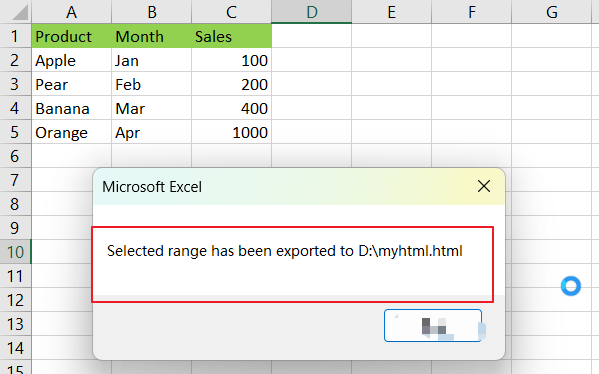
The selected range should now be exported to a text file in the location that you specified.
Video: Export Excel Data to Text Files This
This video will demonstrate how to export Excel data to text files in Excel using VBA Code.
How to Copy Multiple Sheets from Other Workbooks to a New Workbook in Excel
In accounting, statistics or data analysis work, copying worksheets from other workbooks to an existing workbook or to a new workbook is a simple and frequent thing that happens almost every day. Everyone has their own tips or tricks to get around it. This article will describe a common and convenient way to copy all worksheets or some worksheets from other different workbooks into a new one.
Read More: How to Copy a Hidden Sheet to a New Visible Sheet in Excel
Copy Sheets from Other Workbooks to a New Workbook via Move or Copy Feature
Step1: Open the worksheet that contains the sheets you want to copy, and also open the workbook you want to copy those sheets to (if you have such a workbook).
Step2: Hold down the “Ctrl” key on your keyboard and select the worksheet you want to copy to the new workbook.

If you want to copy all the worksheets, hold down the “Shift” key and select the first and the last worksheet, then all the worksheets are selected.

Note that in a Mac workbook you should use the “Command” key instead of the “Ctrl” key.
Step3: Right-click on any of the selected sheets, select “Move or Copy” in the context menu.

Step 4: In “Move or Copy” dialog box, click the drop-down list in “To book” to select a workbook you want to copy to.

Step 5: Select a workbook you want to copy to. You can select an existing workbook or click “(new book)” to create a new workbook. Note that only the opened workbooks are listed in “To book” drop-down list.

Step 6: Select an existing workbook, for example, select “Book 5”, check on “Create a copy“.

Step 7: Click “OK” in “Move or Copy” dialog. The selected worksheets will be copied to the opened existing workbook “Book 5”.

If you select “(New Book)” to copy the selected worksheet, a new workbook will be created and opened and the selected worksheet will be pasted.

Step 8: Repeat above steps to copy sheets from the other workbooks to the destination workbook.
Conclusion
After reading this article, you will know how to select non-consecutive worksheets in a workbook by holding down the “Ctrl” key, and how to create a copy of these selected worksheets in an existing workbook or in a new workbook by using the “Move or Copy” feature. The “Move or Copy” feature helps us move worksheets inside or outside of a workbook in a convenient way and also provides the option to create a copy directly in a specific workbook.
How to Copy a Hidden Sheet to a New Visible Sheet in Excel
If a sheet is hidden, it cannot be accessed or edited directly. By copying it to a new visible sheet, you can access and work with the data on that sheet. Copying a hidden sheet to a visible sheet can also help you create a backup of the hidden sheet. This ensures that you have a copy of the data in case the original sheet becomes corrupted or lost.
This article will show you a great way to copy a hidden worksheet to a new worksheet through VBA code without unhiding or accessing the hidden worksheet.
Copy a Hidden Sheet to a New Visible Sheet Through VBA Code
We may want to hide certain worksheets that contain confidential or sensitive information. If we are the owner of these worksheets, we can copy the hidden worksheet in the traditional way, unhide it and create a copy in the workbook. If we are not allowed to access it, we can still copy the hidden worksheet through VBA code and we can update the data on the new copy without editing the original data.
You can use the following steps to copy a hidden sheet to a new visible sheet using VBA code.
Step1: Open the Excel workbook that contains the hidden sheet and press “Alt+F11” to open the “Visual Basic Editor“. You can also click “Visual Basic” on the “Developer” tab in the ribbon.

Step2: In the “Visual Basic Editor“, right-click on the name of the workbook in the “Project Explorer” and select “Insert > Module” to insert a new module.

Step3: In the module, write the following code:
Sub CopyHiddenSheet()
Sheets("HiddenSheet").Copy Before:=Sheets(1)
Sheets(1).Visible = True
End Sub
In this example, “HiddenSheet” is the name of the hidden sheet that you want to copy. Change it to the name of the hidden sheet that you want to copy.

Step4: Press “F5” or click the “Run” button to run the code.

This will copy the hidden sheet to a new sheet before the first sheet in the workbook and make it visible.

In this step, if you already closed “Visual Basic Editor“, you can also click the “Macros” on the “Developer” tab in the ribbon to run the “Macro“.

Click “Run” in the “Macro” dialog.

Copy a Hidden Sheet with a Different Name Through VBA Code
In this case the code “Sheets(1).Visible = True” works only for the copy of the first worksheet location. It does not work if the copy is saved in a specific location. If you want to copy the hidden worksheet to a specific location, change the “Before:=Sheets(1)” parameter to the desired worksheet location.
For example, if you want to copy the hidden worksheet to the end of the workbook, change it to “After:=Sheets(Sheet.Count)“. If you want to create a copy after the hidden sheet, change it to “After:=Sheets(“HiddenSheet”)“. This operation will only copy the sheet to a specific location, but will not set it to be visible.
If you want to copy the hidden sheet with a different name, you can write the following code.
Sub CopyHiddenSheet()
Sheets("HiddenSheet").Copy Before:=Sheets(1)
Sheets(1).Visible = True
Sheets(1).Name = "New Sheet Name"
End Sub
Here, for the “New Sheet Name“, change it to the name you want to name the copy hidden sheet.

Conclusion
After reading this post, you have gained the skills to copy hidden worksheets to visible worksheets by editing VBA code. With Visual Basic editor, you can see all visible and invisible worksheets. By editing the provided code, you can copy the worksheet you want to copy to any specific location. You can also rename the copied worksheet correctly with the VBA code.
How to Quickly Copy the Every Other Row in Excel Worksheet
In some cases, you may want to perform data analysis on every other row in a table, such as calculating averages or performing other calculations. By copying every other row, you can quickly create a new table with the necessary data for analysis.
For example, suppose there are multiple rows in a spreadsheet and we want to extract only the odd or even rows.

In fact, extracting odd or even rows is equivalent to copying every other row in the original table to a new location. This post will show you some ways to copy every other row to another location in Excel. After reading this post, you can choose anyone to apply it in your daily work.
Read More: Copy Non-Adjacent Cells or Columns or Rows in Excel
Copy The Every Other Row by Traditional Copy and Paste Features
If you only have a few rows to extract and copy to another location, you can simply use the traditional copy and paste function by pressing the “Ctrl” key to select the multiple rows you want to copy.
Here are the steps:
Step 1: Select the first line that you want to copy. In this example, select the range A1:B1.

Step 2: Hold down the “Ctrl” key and select every other odd row that you want to copy.

Step 3: Press “Ctrl + C” on your keyboard to copy the selected odd rows.

Step 4: Select the first cell in the new location where you want to paste the copied rows.

Step 5: Right-click on the selected cell and choose “Paste” from the menu. You can also press “Ctrl + V” on your keyboard to paste the selected rows.

In this way, the selected rows are copied to the new location, and the copied rows are not separated.

Copy The Every Other Row by Filter Function
We can also copy every other row in a table to another location with the Filter function. We need to create a helper column to help us achieve it. Here are the specific steps.
Step 1: Create a helper column in column C. Populate the value “0” to the odd rows and the value “1” to the even rows.

Step 2: Select the helper column and click the “Filter” button on the “Data” tab in the ribbon.

Step 3: Click the dropdown arrow in the column header of the helper column that contains “0” and “1” numbers.

Step 4: Filter by value “0” and apply the filter. Then only the odd number rows are visible. The even number rows are hidden.

Step 5: Select the filtered rows, press “Ctrl + C” to copy the selected rows.

Step 6: Select the first cell in the new location and press “Ctrl + V” to paste the selected row. You may find that some rows are invisible because they are hidden.

Step 7. Click on “Filter” in the ribbon to clear the filter. All hidden rows are unhidden and visible. The selected rows are copied correctly to the new location.

Copy The Every Other Row by Fill Handle
If you want to keep a blank row between each selected row to keep the table structure unchanged, you can refer to the following steps.
Step 1: Create a simple formula “=A1” in cell D1.

This formula will help us copy the value of A1 to the currently selected cell.

Step 2: Keep D1 selected. Drag the handle to fill the formula to cell E1.

Due to the location change, the formula is updated to “=B1“.

Step 3: Select the range D1:E2. This range contains two short rows, row1(D1:E1) is the row copied from the original table by the fill formula and row2 is a blank row which is used to separate the copied rows.

Step 4: Drag the handle down so that the following rows are filled with reference to the rule. In this way, not only the values, but also the structure of the table is copied to the new location.

Conclusion
Copying every other row in Excel is a useful technique in a variety of situations, such as filtering data and data analysis. It can help simplify the process of working with large data sets and can make it easier to spot outliers in the data. You can choose the appropriate way to copy the every other row in Excel depending on the specific task at hand and the requirements of the project or analysis.
How to Export a Range of Data to HTML or Web Page File in Excel
This post will explain how to export a range of data from an Excel worksheet to an HTML or web page file using the Save As command and VBA code. This method allows you to create a standalone HTML file that can be opened in any web browser, making it easy to share your data with others.
Export a Range of Data to HTML or Web Page File with Save As Command
If you want to export a range of data from Excel to HTML or web page file, one common method is to use the “Save As” function in Excel.
Here are the steps:
Step1: Select the range of data you want to export to HTML. You can select the cells by clicking and dragging the cursor over the cells.

Step2: Click on the “File” tab in the Excel ribbon. Click on “Save As“.

Step3: In the “Save As” dialog box, choose “Web Page” from the file type dropdown menu. Choose the location where you want to save the file and give it a name. Click on “Publish” button.

Step4: In the “Publish Options” section, select the “Selection” option to export only the selected range of cells. click Save button.

Step5: the Publish as Web Page dialog box will open, Click on the “Publish” button to export the range of data to an HTML file.

Step6: After completing these steps, the selected range of data will be exported to an HTML file that can be opened in a web browser.
Export a Range of Data to HTML or Web Page File with VBA Code
You can also export a range of data to an HTML file with VBA Code in Excel, and you can use the Application.InputBox function to select the range of data to export and prompt the user to select the destination directory and filename. Just do the following steps:
Step1: Press ALT + F11 on your keyboard to open the Visual Basic Editor (VBE).

Step2: In the VBE, click on the Insert menu and select Module. This will create a new module in your VBA project.

Step3: Copy the below VBA code and paste it into the module. Save your VBA project and close the VBE.

Sub ExportRangeToHTML_Excelgeek()
Dim wb As Workbook
Dim ws As Worksheet
Dim rng As Range
Dim htmlFile As String
Set wb = ThisWorkbook
Set ws = wb.ActiveSheet
' Prompt the user to select the range of data to export
Set rng = Application.InputBox(prompt:="Select the range of data to export as HTML", Type:=8)
' Prompt the user to select the destination directory and filename
htmlFile = Application.GetSaveAsFilename(fileFilter:="HTML Files (*.html), *.html")
'Create a new workbook with the selected range of data and save it as an HTML file
Dim newWb As Workbook
Set newWb = Workbooks.Add
rng.Copy
newWb.Sheets(1).Range("A1").PasteSpecial xlPasteAll
newWb.SaveAs htmlFile, xlHtml
newWb.Close
MsgBox "Selected range has been exported to " & htmlFile
End Sub
Step4: Press ALT + F8 on your keyboard to open the Macro dialog box. Select the ExportRangeToHTML_Excelgeek macro from the list and click the Run button.

Step5: select the range of data to export in your current worksheet.

Step6: choose a location to save the HTML file.

Step7: Once the macro has completed, a message box will appear indicating that the selected range has been exported to the chosen location.

You should now have an HTML file containing the data from the selected range.
Conclusion
Now you can quickly and easily export a range of data to an HTML file without having to manually copy and paste the data into a web page editor.
How to Copy Non-Adjacent Cells or Columns or Rows in Excel
When you are working with a large dataset in a Excel spreadsheet, you may need to copy non-adjacent cells or columns or rows to perform various analyses, such as comparing data from different columns or rows. In this article, we will describe the method of copying non-adjacent cells or columns or rows in a worksheet.
Read More: Copy Cell Formatting from a Given Cell to Another Cell or a Range
Copy Non-Adjacent Cells in Excel Worksheet
Excel does not support copying multiple non-adjacent cells from different rows or columns, a warning message pops up when copying the non-adjacent cells. So in this example, we only copy non-adjacent cells in the same row or column to explain the method.

To copy non-adjacent cells in Excel, you can follow these steps:
Step1: Select the first cell you want to copy, for example, click on cell A2. Hold down the “Ctrl” key on your keyboard.

Step2: While still holding down the “Ctrl” key, select the other cells that you want to copy.

Step3: Once you have selected all the cells that you want to copy, release the “Ctrl” key.
Step4: Right-click on any of the selected cells and click on “Copy” or press “Ctrl + C” on your keyboard.

Step5: Select the cell where you want to paste the copied cells.
Step6: Right-click on the cell and click on “Paste” or press “Ctrl + V” on your keyboard. After this step, the selected non-adjacent cells are copied and pasted to another location properly.

Copy Non-Adjacent Rows or Columns in Excel Worksheet
You can also follow the steps below to copy non-adjacent rows or columns to another location in worksheet.
Step1: Select the first row or column that you want to copy by clicking on its header (the letter or number at the top or left of the row or column). In this example, click on the first column header “A” to select the entire column.
Step2: Hold down the “Ctrl” key on your keyboard and select the other rows or columns that you want to copy. You can select as many non-adjacent rows or columns as you want.
In this example, hold down the “Ctrl” key and select both column C and column D by dragging the mouse.

Step3: Once you have selected all the rows or columns that you want to copy, right-click on any of the selected rows or columns and choose “Copy” from the context menu.

Step4: Navigate to the location in the worksheet where you want to paste the copied rows or columns.
Step5: Right-click on the cell where you want to start the paste and choose “Paste” from the context menu.

The copied non-adjacent columns will be pasted into the new location.

Conclusion
Overall, you can use the normal copy and paste features to copy non-adjacent rows or columns. Just make sure to hold down the “Ctrl” key while selecting the rows or columns you want to copy, and while clicking on the cell where you want to start the paste.
How to Reference Formatting and Value from Another Cell with Same Size, Font and Style in Excel
Except Copy & Paste method to copy a value from another cell, we can also copy the value we want to copy by using its cell reference, for example, if the value is saved in cell A1, we can build a formula “=A1” to copy the value. However, this method only supports copying values from another cell, while ignoring the formatting, size and font.
Read More: Copy Cell Formatting from a Given Cell to Another Cell or a Range
If we want to duplicate cells with exactly the same size, font, formatting and values, we must consider other methods to achieve it. This post provides the way to make the copied cells with the same reference format.

Reference Formatting and Value from Another Cell by Excel Paste Special Feature
To reference formatting and value from another cell by Excel Paste Special, you can follow these steps:
Step1: Select the cell you want to copy the formatting and value from. In this example, the cell is A1.
Step2: Press Ctrl+C to copy the cell.
Step3: Select the cell you want to apply the formatting and value to. In this example, we select C1 to create a copy.
Step4: Right-click on the selected cell and choose “Paste Special” -> “Paste Picture Link” from the menu.

Step5: After all the formatting and value are applied to the selected cell(s).

The “Paste Special” function can be used for a variety of purposes, including copying formulas, comments, validation, and more. Make sure you select the appropriate method in the “Paste Special” menu for the desired effect.

You can see that we can get a duplicate cell by “Paste Picture” method as well. Actually, in Excel, “Paste Picture” and “Paste Picture Link” are two different options for pasting a picture into a worksheet.
“Paste Picture” will insert a copy of the picture into the worksheet, and the picture will be embedded in the worksheet. The picture will be visible even if the original source file is deleted or moved.
“Paste Picture Link” will insert a link to the picture into the worksheet, rather than embedding the picture itself. If the original picture file is moved or deleted, the picture in the worksheet will not be visible and will display a broken link icon.
How to Copy Only Formatting from a Range to Another Range in Excel
When you want to ensure consistency in the formatting of a range of cells, copying only the formatting can be helpful. For instance, if you have a large spreadsheet with several rows and columns, you may want to ensure that all the cells have the same font, size, and color, which can be achieved by copying the formatting from one range to another. And copying formatting is a great time saver, it avoids errors when manually adjusting fonts and styles.
See the example below. We want the two “SALES” columns have the same range formatting. This post shares three methods including VBA code to copy only formatting from one range to another in Excel worksheet.

Copy Only Formatting from a Range to Another by Format Painter Tool
Format Painter is useful in Excel and it can copy the style and formatting from a cell or a range and apply it on your destination cell or range in a quick way.
You can copy only the formatting from one range to another range by Format Painter tool in Excel by the following steps:
Step1: Select the cell that has the formatting you want to copy. In this example, the source range is B4:B8 which contains one number format and two background colors in cells.
Step2: Click on the “Format Painter” button in the “Home” tab of the Excel ribbon. The cursor will change to a paintbrush.

Step3: Select the range of cells that you want to apply the formatting to. The copied range’s formatting will be applied to the entire destination range.

Copy Only Formatting from a Range to Another by Paste Special -> Formatting Feature
You can also copy only formatting from a range to another by Excel “Paste Special” feature, this feature contains several “Paste” methods, and “Formatting” which copies only formatting and ignores the contents.
Here are the steps:
Step1: Select the cell or range that contains the formatting you want to copy.
Step2: Press “Ctrl + C” or right-click the selection and choose “Copy” from the context menu.
Step3: Select the cell or range where you want to apply the formatting.
Step4: Right-click the selection and choose “Paste Special” -> “Formatting” from the context menu.

This will copy only the formatting from the original range to the destination range.
Copy Only Formatting from a Range to Another by Excel VBA Module
If you are familiar with Excel VBA, you can also copy only formatting from a range to another range in Excel using VBA code. Here are the steps:
Step1: Press Alt+F11 or click Visual Basic in Develop tab to open the Visual Basic Editor.

Step2: In the VBE, select the opened sheet you want to run the VBA code, select “Insert” from the menu bar, then choose “Module“.

Step3: Create VBA code.

a. Define the source range and destination range by declaring two range variables using the “Range” object in VBA.
b. Use the “Copy” method of the source range object to copy the formatting only. This can be done by setting the “Paste Special” method to paste only the formatting.
c. Clear the clipboard to remove any copied data by using the “Application.CutCopyMode” method.
The complete VBA code should look like this:
Sub CopyFormattingOnly()
Dim rngSource As Range
Dim rngDestination As Range
Set rngSource = Range("A1:D10") 'Change to your desired source range
Set rngDestination = Range("F1:I10") 'Change to your desired destination range
rngSource.Copy
rngDestination.PasteSpecial xlPasteFormats
Application.CutCopyMode = False
End Sub
Step4: Save the VBA code, close the editor and go back to the worksheet.
Step5: To run the macro, press Alt+F8 to open the Macro dialog box or click Macros in Developer tab.

Step6: Select the macro you just created and click the Run button.

Step7: After running the macro, the destination range is applied with the formatting properly.

How to Format Ranges with the Same Formatting from Another Cell in Excel
Copying cell formatting from another cell and apply on another range or some ranges can be useful in several scenarios. It can save time, ensure consistency, and reduce the chance of errors when working with large sets of data in Excel. This post shares two tips to format ranges as same as the format from another cell in the Excel worksheet.
Read More: Copy the Specified Cell Formatting to Another Cell or Cells
Example.

Format Ranges from Another Cell’s Formatting by Format Painter Tool
You can use the “Format Painter” tool in Excel to apply the same formatting from one cell to a range of cells.
Here are the steps:
Step1: Select the cell that has the formatting you want to copy. In this example, you can select cell “B2” or any cell in the range “B5:B9” that has the same cell format.
Step2: Click on the “Format Painter” button in the “Home” tab of the Excel ribbon. The cursor will change to a paintbrush.

Step3: Select the range of cells that you want to apply the formatting to. The copied cell’s formatting will be applied to the entire range.

Format Ranges from Another Cell’s Formatting by “Paste Special” Feature
Alternatively, you can also use the “Paste Special” feature to apply formatting from one cell to a range of cells. “Special Paste” -> “Format” enables you to copy the cell style and formatting from another cell and paste it into the target cell or cell area without copying the values and formulas.
Here are the steps:
Step1: Select the cell that has the formatting you want to copy. You can select cell B2 in this example because it contains the style and format for a price.
Step2: Press “Ctrl+C” to copy the cell.
Step3: Select the range of cells that you want to apply the formatting to. In this example, select the range E5:E9 where you want to keep consistency with the price’s format.
Step4: Right-click on the selection and choose “Paste Special“-> “Formatting” from the context menu. The formatting from the original cell will be applied to the entire range.

Conclusion
Formatting a range as same as a given cell’s formatting is easily achieved by above two ways. After running the above steps, the values in the SALES column match the style and formatting of cell B2. You can choose either one you like to format your ranges in work.