How to Copy and Paste Cell Data Including Row Height and Column Width in Excel

If we want to copy a cell with different size to another normal size cell, its content will not be fully displayed in the destination with the desired size. Copying data with cell dimensions, including row heights and column widths, will ensure that the pasted cells are the same size as the copied cells, which will help us check the data in the spreadsheet for a good and consistent table structure.

Read More: Copy and Paste Cell or Row Heights to Another in Excel

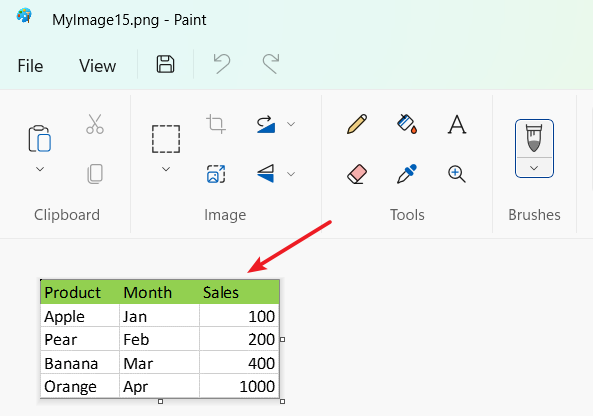
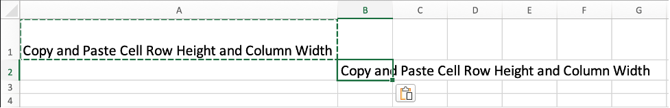
If we copy the cell only by traditional “Copy “and “Paste” features, only the cell value is copied to the destination.

How to Copy and Paste Cell Data Including Row Height and Column Width in Excel 1.png

Our goal is to copy and paste calls that include not only their cell values, but also cell dimensions, such as row height and column width. This post will show you the way to copy and paste cell with its row height and column width in Excel.

Copy and Paste Cell Row Height and Column Width via Excel Paste Special Feature and Format Painter Feature

In Excel worksheet, to copy and paste cell data including the cell row height and column width, you can follow these steps:

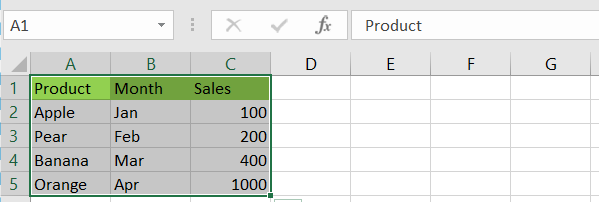
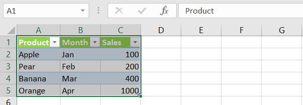
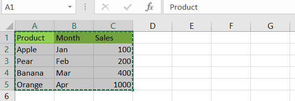
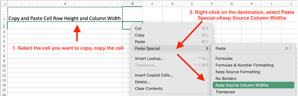
1. Select the cell or range of cells that you want to copy.

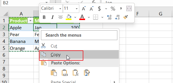
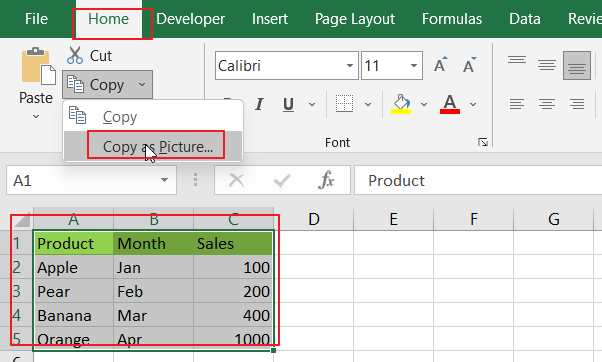
2. Right-click on the selected cell, select “Copy” in the menu. Or press “Ctrl + C” on your keyboard.

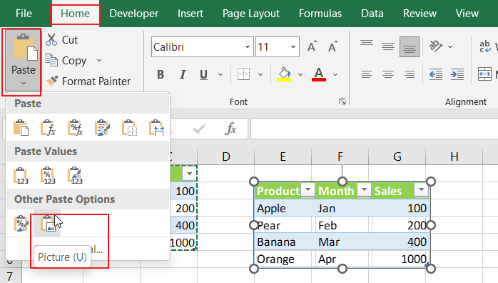
3. Select the destination cell or range of cells where you want to paste the copied data.

4. Right-click on the destination cell or range of cells and select “Paste Special” -> “Keep Source Column Widths” from the “Paste Special” menu.

How to Copy and Paste Cell Data Including Row Height and Column Width in Excel 2.png

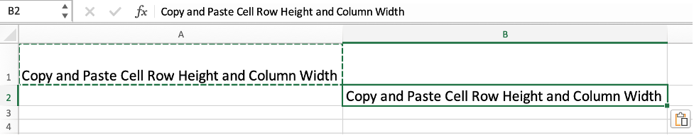
After this step, column widths are applied to the selected cell or range of cells properly.

How to Copy and Paste Cell Data Including Row Height and Column Width in Excel 3.png

The following are the steps for copying the row height:

5. Click on the row number of the row that you want to copy the row height.

How to Copy and Paste Cell Data Including Row Height and Column Width in Excel 4.png

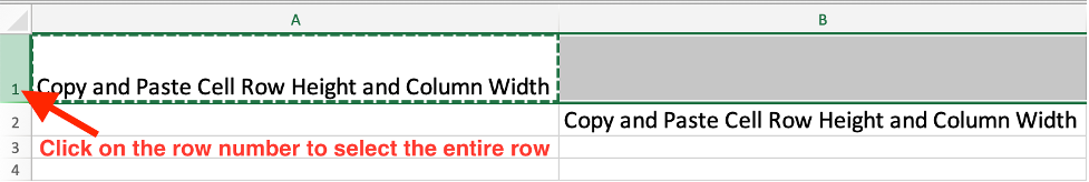
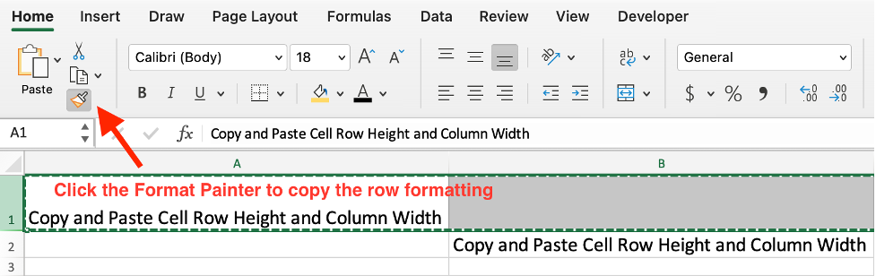
6. Click the Format Painter on the Home tab of the ribbon.

How to Copy and Paste Cell Data Including Row Height and Column Width in Excel 5.png

7. Click on the row number of the row that you want to apply the row height. Format Paint will apply the row height to the selected row.

How to Copy and Paste Cell Data Including Row Height and Column Width in Excel 6.png

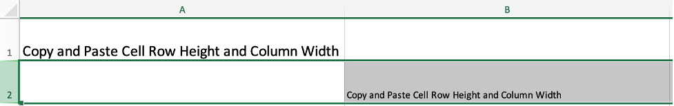
Note: After copying the row height with the Format Paint tool, the font size is reduced to 12, which is the default font size when opening an Excel worksheet. This is because the default font size for row 1 is still 12 (cell A1 has a font size of 18), and when copying the row formatting, the default font size is applied to the selected row as well. So it is better to copy the row height first, and then copy the cell values while maintaining the

How to Copy and Paste Cell or Row Heights to Another in Excel

Sometimes we need to adjust the row heights in our worksheets to ensure that consistent row heights can make Excel spreadsheets look more organized and visually appealing. If the rows are not evenly sized, the data may not align properly and can make it difficult to read. In this post, we will introduce some ways to copy the row height in an Excel worksheet to another row.

Read More: Copy and Paste Cell Sizes to Another Worksheet or Workbook in Excel

Copy and Paste Row Heights via Copying the Row Height Value

You may have tried to copy the row heights through Excel’s special paste feature. There is no such option to paste the row heights, only the column widths included.

By checking the row height in Excel, you can copy the row height number and copy it to the row height when you adjust another row. You can do this by following these steps.

Step1: Select the row(s) whose height you want to check. You can do this by clicking on the row number on the left-hand side of the worksheet.

How to Copy and Paste Cell or Row Heights to Another in Excel 1.png

Step2: Right-click on the selected row(s) and click on “Row Height” in the context menu.

How to Copy and Paste Cell or Row Heights to Another in Excel 2.png

Step3: In the “Row Height” dialog box, the “Row height” field will display the row height. In this example, the row height is “60”, you can also change the row height in this dialog box if you need to.

Step4: Copy the “Row height” number and click “OK” to close the dialog box.

How to Copy and Paste Cell or Row Heights to Another in Excel 3.png

Step5: Select another row whose height you want to pasted the row height. Click on the row number to select the entire row.

Step6: Right-click on the selected row(s) and click on “Row Height” in the context menu. Before copying the row height, the current row height is displayed in row height field.

How to Copy and Paste Cell or Row Heights to Another in Excel 4.png

Step7: Press “Ctrl+V” to paste the row height value we copied from row 1.

How to Copy and Paste Cell or Row Heights to Another in Excel 5.png

After all above steps, row height is copied and applied to row 2 properly.

How to Copy and Paste Cell or Row Heights to Another in Excel 6.png

Copy and Paste Row Heights via Using the Format Painter

Another way to check the row height is to use the “Format Painter” tool. Here are the steps:

Step1: Click on the row number to select the row whose height you want to copy.

How to Copy and Paste Cell or Row Heights to Another in Excel 7.png

Step2: Click on the “Format Painter” button in the “Home” tab of the Excel ribbon.

How to Copy and Paste Cell or Row Heights to Another in Excel 8.png

Step3: Click on another row number to apply the copied row height. The height of the selected row will change to match the height of the copied row, allowing you to visually compare the two row heights.

How to Copy and Paste Cell or Row Heights to Another in Excel 9.png

Conclusion

In summary, checking row height can help make your Excel spreadsheets more visually appealing, easier to read, and more functional for various tasks such as printing, filtering, sorting, and merging cells. After reading the post, you can adjust your row heights in a more convenient and accurate way to keep them consistent.

How to Copy and Paste Cell Sizes to Another Worksheet or Workbook in Excel

If you have a table or worksheet where you have already set up the column widths and row heights to your desired dimensions, you can use the copy and paste technique to quickly apply the same sizes to other cells or ranges, or even other worksheets or workbooks. This can help maintain a consistent and professional appearance throughout the worksheet or workbook.

In this post, we introduced some ways to copy and paste cells to the destination in another worksheet or workbook by copying the column width or row height as well. Let’s get started.

Read More: Copy and Paste Cell or Row Heights to Another in Excel

Copy and Paste Cell Column Widths in Another Worksheet or Workbook

When copying a table to a location in another worksheet or workbook via the traditional copy and paste function, only the values are copied to the destination, without copying the formatting, style or size, etc.

If a table with wide column widths is copied to a location with only narrow column widths, the copied values are not fully displayed in the columns and we must manually adjust the column widths.

How to Copy and Paste Cell Sizes to Another Worksheet or Workbook in Excel

In fact, we can now paste the copied table via “Special Paste” -> “Function” and include the column width correctly.

Here are the steps.

Step1: Select the cells whose sizes you want to copy.

Step2: Right-click on the selected cells and choose “Copy” from the context menu, or press “Ctrl+C” on your keyboard.

Step3: Select the destination cells where you want to paste the sizes. You can select a single cell, a range of cells, or even an entire row or column.

Step4: Right-click on the destination cells and choose “Paste Special” -> “Keep Source Column Widths” from the context menu.

How to Copy and Paste Cell Sizes to Another Worksheet or Workbook in Excel

Or press “Ctrl+Alt+V” on your keyboard to open “Paste Special” dialog box, and check on “Column widths” checkbox, and click “OK” to apply the changes.

How to Copy and Paste Cell Sizes to Another Worksheet or Workbook in Excel

Copy and Paste Cell Column Widths and Row Heights in Another Worksheet or Workbook

When copying and pasting cells, there is no such a way to allow copying the row height. But we can still do it in a special way.

Here are the steps:

Step1. Open the worksheet that contains the table you want to copy.

Step2. Click on the worksheet tab at the bottom of the screen to activate it.

Step3. Click on the “Select All” button located at the top-left corner of the worksheet, where the column and row headers meet. This selects all cells in the worksheet.

How to Copy and Paste Cell Sizes to Another Worksheet or Workbook in Excel

Step4. Right-click on any selected cell and choose “Copy” from the context menu, or press “Ctrl + C” on your keyboard.

Step5. Click on the worksheet tab or workbook where you want to paste the copied cells.

Step6. Click on the “Select All” button, press “Ctrl + V” to copy all cells with cell sizes from source worksheet to the new worksheet. In this way, the column widths and row heights are copied correctly to their destinations in the desired dimensions.

How to Copy and Paste Cell Sizes to Another Worksheet or Workbook in Excel

How to Copy a Selected Range to New Workbook in Excel

If you work with large amounts of data in Excel, it is likely that you have needed to copy a selected range of cells to a new workbook at some point. While you can manually copy and paste the range, this process can be time-consuming and error-prone, especially if you need to repeat the task frequently.

Fortunately, there are several ways to automate the process of copying a selected range to a new workbook in Excel. In this post, we will introduce two methods to achieve this task – the first one is the manual method, and the second one is using VBA code with Application.InputBox to select the range.

Copy a Selected Range to a New Workbook Manually

If you want to copy a selected range to a new workbook manually in Excel , you can follow these steps:

Step1: Select the range of cells you want to copy.

How to copy a selected range to a new workbook in Excel1.png

Step2: Press Ctrl + C on your keyboard to copy the selected range.

Step3: Click on the File tab in the ribbon menu, then select New to create a new workbook.

Step4: In the new workbook, click on the first cell where you want to paste the copied range.

How to copy a selected range to a new workbook in Excel2.png

Step5: Press Ctrl + V on your keyboard to paste the copied range.

Copy a Selected Range to a New Workbook with VBA Code

You can also use the VBA Code to copy a selected range to a new workbook in Excel, it will use the Application.Inputbox function to select the range. Just do the below steps:

Step1: Open the Excel workbook that contains the range you want to copy.

Step2: Press Alt + F11 on your keyboard to open the Visual Basic Editor.

Step3: In the Visual Basic Editor, click on Insert from the top menu and select Module to insert a new module.

Step4: Copy and paste the VBA code provided in the module.

vba to copy a selected range to a new workbook in Excel1.png
Sub CopyRangeToNewWorkbook_excelgeek()
    Dim myRange As Range
    Dim newWorkbook As Workbook
    
    'Prompt user to select range to copy
    Set myRange = Application.InputBox(prompt:="Select the range to copy", Type:=8)
    
    'Create a new workbook
    Set newWorkbook = Workbooks.Add
    
    'Copy the selected range to the new workbook
    myRange.Copy Destination:=newWorkbook.Sheets(1).Range("A1")
    
    'Activate the new workbook
    newWorkbook.Activate
End Sub

Step5: Press F5 or Run from the top menu to run the macro.

vba to copy a selected range to a new workbook in Excel2.png

Step6: In the pop-up window, select the range you want to copy by clicking and dragging your mouse over the cells. Click on the OK button to start the macro.

vba to copy a selected range to a new workbook in Excel3.png

Step7: Excel will create a new workbook and copy the selected range to the new workbook.

vba to copy a selected range to a new workbook in Excel4.png

How to Save an Excel Table as Image in Excel

This tutorial will introduce three methods for saving an Excel table as an image in Excel: “Paste as picture”, “Paint tool”, and “VBA code“.

The Paste as picture method allows you to create a picture of a range that can be easily inserted into documents or presentations.

The Paint tool method uses the built-in Windows Paint program to save the selected range as an image.

The VBA code method automates the process of saving the selected range as an image using Visual Basic for Applications (VBA) code.

Save Table as Image using Paste as Picture

You can save an Excel table as an image using the “paste as picture” feature. Here are the steps:

Step1: Select the table that you want to save as an image.

How to Save an Excel Table as Image in Excel 1.png

Step2: Right-click on the selected cells and choose “Copy” from the context menu or press Ctrl+C on your keyboard.

How to Save an Excel Table as Image in Excel 2.png

Step3: select one destination cell to place the image.  Then click the Home tab, click on the drop-down menu list from the Paste option in the Clipboard group.  Click on the Picture option.

How to Save an Excel Table as Image in Excel3.png

Now you can simply copy the image and paste it to other application.

Save Table as Image using Paint Tool

You can save an Excel table as an image using the Paint tool in Windows. Here are the steps:

Step1: Select the table that you want to save as an image.

Step2: Right-click on the selected cells and choose “Copy” from the context menu or press Ctrl+C on your keyboard.

Step3: Open the Paint tool by typing “Paint” in the Windows search bar and selecting the app from the search results.

Step4: In Paint, choose “Paste” from the “Home” tab or press Ctrl+V on your keyboard to paste the copied table into the canvas.

How to Save an Excel Table as Image in Excel4.png

Step5: Choose “Save As” from the “File” menu and select the desired file format (e.g. JPEG, PNG, BMP, etc.).

How to Save an Excel Table as Image in Excel5.png

Step6: Enter a file name and choose a save location. Click “Save” to save the image.

How to Save an Excel Table as Image in Excel6.png

Save Table as Image with VBA Code in Excel

You can use VBA code in Excel to save a selected table as an image and prompt the user to select a destination to save the image. Just do the following steps:

Step1: Open your Excel workbook.

Step2: Press Alt + F11 to open the VBA editor.

Step3: In the VBA editor, select Insert from the menu bar, then choose Module to create a new module.

Step4: Copy the VBA code I provided and paste it into the new module. Save the workbook and close the VBA editor.

vba to Save an Excel Table as Image in Excel 1.png
Sub sleep(T As Single)
    Dim time1 As Single
    time1 = Timer
    Do
        DoEvents
    Loop While Timer - time1 < T
End Sub
Sub SaveTableAsImage_excelgeek()
    Dim tbl As Range
    Dim savePath As String, fileName As String, fileFormat As String
    Dim cht As ChartObject
      
    'Prompt the user to select the table to save as an image
    Set tbl = Application.InputBox("Select the table to save as an image:", Type:=8)

    tbl.CopyPicture xlScreen, xlPicture
 
     'prompt user for save location and file name
    savePath = Application.GetSaveAsFilename(InitialFileName:="table1", _
        FileFilter:="JPEG (*.jpg), *.jpg, PNG (*.png), *.png")
    If savePath = "False" Then Exit Sub ' exit if user clicks cancel
     
    'extract file name and format from save path
    fileName = Mid(savePath, InStrRev(savePath, "\") + 1)
    fileFormat = Mid(fileName, InStrRev(fileName, ".") + 1)
    fileName = Left(fileName, InStrRev(fileName, ".") - 1)
    
    
    'create temporary chart object, set dimensions to table dimensions, paste table inside, and save as image
    Set cht = ActiveSheet.ChartObjects.Add(0, 0, tbl.Width, tbl.Height)
    Call sleep(2)
    cht.Chart.Paste
    cht.Chart.Export savePath, fileFormat
    cht.Delete
    Application.CutCopyMode = False
    
End Sub

Step5: Press Alt + F8 to open the Macros dialog box. Select the SaveTableAsImage_excelgeek macro from the list and click the Run button.

vba to Save an Excel Table as Image in Excel 2.png

Step6: Select the table to save as an image.

vba to Save an Excel Table as Image in Excel 3.png

Step7: select one the location to place image.

vba to Save an Excel Table as Image in Excel 4.png

Step8: The picture will be saved into the selected location.

vba to Save an Excel Table as Image in Excel 5.png

Conclusion

There are several methods available for saving an Excel table as an image, each with its own advantages and limitations. The “Paste as picture” method is quick and easy, but may result in lower image quality. The “Paint tool” method provides greater control over image quality, but requires an extra step. The “VBA code” method offers the most automation and customization options, but may require some programming knowledge.

How to Copy and Paste Range or Chart object as Picture in Excel

This post will introduce two methods to copy and paste a range or chart object as a picture in Excel. The first method involves using Excel’s built-in “Copy as Picture” feature, while the second method uses VBA code to automate the process.

The VBA code method will select a range or chart object using Application.Inputbox function and choose a destination cell for the picture. The VBA code will then copy the range or chart object as a picture and paste it into the specified cell.

Copy and Paste Range or Chart object as Picture using Copy as Picture

You can use the “Copy as Picture” feature in Excel to copy a range or chart object as a picture. Here are the steps:

Step1: Select the range or chart object that you want to copy as a picture.

How to Copy and Paste Range or Chart object as Picture in Excel 1.png

Step2: Go to the “Home” tab in the Excel Ribbon. Click the drop-down arrow next to the “Copy” button in the “Clipboard” section. Select “Copy as Picture” from the drop-down menu. The Copy Picture dialog box will open.

How to Copy and Paste Range or Chart object as Picture in Excel 2.png

Step3: In the “Copy Picture” dialog box, select the Format as Picture, and select Appearance as shown on screen.

How to Copy and Paste Range or Chart object as Picture in Excel 3.png

Step4: Click the “OK” button to copy the range or chart object as a picture.You can paste the picture wherever you want by pressing “Ctrl + V” on the keyboard.

How to Copy and Paste Range or Chart object as Picture in Excel 4.png

Copy and Paste Range or Chart object as Picture with VBA Code

You can also use the VBA Code to copy a range or chart object and paste it in your Excel worksheet, just do the following steps:

Step1: Open your Excel workbook.

Step2: Press Alt + F11 to open the VBA editor.

Step3: In the VBA editor, select Insert from the menu bar, then choose Module to create a new module.

Step4: Copy the VBA code I provided and paste it into the new module. Save the workbook and close the VBA editor.

vba Copy and Paste Range or Chart object as Picture in Excel 12.png
Sub CopyAsPicture_excelgeek()
    Dim rng As Range
    Dim chartObj As ChartObject
    Dim destCell As Range
    
    'Prompt user to select range or chart object
    On Error Resume Next
    Set rng = Application.InputBox("Select a range or chart object to copy as picture", Type:=8)
    On Error GoTo 0
    
    'If user selects a range, copy it as picture
    If Not rng Is Nothing Then
        rng.CopyPicture xlScreen, xlPicture
        
        'Prompt user to select destination cell
        On Error Resume Next
        Set destCell = Application.InputBox("Select destination cell to place picture", Type:=8)
        On Error GoTo 0
        
        'If user selects a cell, paste the picture and adjust its size
        If Not destCell Is Nothing Then
            With destCell.Parent.Pictures.Paste
                .Left = destCell.Left
                .Top = destCell.Top
                .Width = rng.Width
                .Height = rng.Height
            End With
        End If
    'If user selects a chart object, copy it as picture
    ElseIf ActiveChart Is Nothing Then
        MsgBox "Please select a range or chart object."
    Else
        Set chartObj = ActiveSheet.ChartObjects(ActiveChart.Parent.Name)
        chartObj.Chart.Export Environ$("temp") & "\temp.png", "PNG"
        With destCell.Parent.Pictures.Insert(Environ$("temp") & "\temp.png")
            .Left = destCell.Left
            .Top = destCell.Top
            .Width = chartObj.Width
            .Height = chartObj.Height
        End With
        Kill Environ$("temp") & "\temp.png"
    End If
End Sub

Step5: Press Alt + F8 to open the Macros dialog box. Select the CopyAsPicture_excelhow macro from the list and click the Run button.

vba Copy and Paste Range or Chart object as Picture in Excel 13.png

Step6: Select the cell where you want to paste the picture.

vba Copy and Paste Range or Chart object as Picture in Excel 3.png

Step7: select one the destination cell to place picture.

Step8: The picture will be pasted into the selected cell.

vba Copy and Paste Range or Chart object as Picture in Excel 5.png

How to Convert Range to Image in Excel

This post will introduce you to two methods of converting a range of cells to an image in Excel. The method involves using the “Copy As Picture” feature in Excel and a VBA code to export the copied range as an image file.

Convert Cells Range to Image Using Copy as Picture Feature

If you want to convert a range of cells to an image in Microsoft Excel Spreadsheet, you can use the built-in “Copy As Picture” feature. Here are the steps:

Step1: Select the cells range that you want to convert to an image.

Step2: Press the “Ctrl + C” shortcut on your keyboard to copy the cells range to the clipboard.

How to convert cells range to image in Excel 1.png

Step3: Click on the “Home” tab in the ribbon. Click on the “Copy” dropdown arrow in the “Clipboard” group, and then select “Copy as Picture“. The Copy Picture dialog box will open.

How to convert cells range to image in Excel 2.png

Step4: In the “Copy Picture” dialog box, select the “As shown on screen” option and the “Picture” format. Click on the “OK” button.

How to convert cells range to image in Excel 3.png

Step5: Now you can paste the copied cells range as an image in another location. For example, you can open an image editor (such as Microsoft Paint), and press the “Ctrl” and “V” keys on your keyboard to paste the image.

How to convert cells range to image in Excel4.png

Convert Cells Range to Image with VBA Code

You can also use VBA code to automate the process of converting a range of cells to an image. Just do the following steps:

Step1: Open your workbook that contains the range of cells you want to convert to an image.

Step2: Press Alt + F11 to open the Visual Basic Editor.

Step3: In the Visual Basic Editor, click on Insert > Module to create a new module.

Step4: Copy the below VBA code and paste it into the new module.

vba to convert cells range to image in Excel 1.png
Sub ConvertRangeToImage_excelgeek()
    Dim MyChart As ChartObject
    Dim MyRange As Range
    Dim DestPath As String
    Dim FileName As String
    
    Set MyRange = Application.InputBox("Select the range of cells:", Type:=8)
    MyRange.CopyPicture xlScreen, xlPicture
    
    Set MyChart = ActiveSheet.ChartObjects.Add(0, 0, MyRange.Width, MyRange.Height)
    
    MyChart.Activate
    MyChart.Chart.Paste
    DestPath = Application.GetSaveAsFilename(InitialFileName:="MyImage", _
        FileFilter:="PNG Files (*.png), *.png, JPEG Files (*.jpg), *.jpg, GIF Files (*.gif), *.gif, BMP Files (*.bmp), *.bmp", _
        Title:="Save As")
    If DestPath <> "False" Then
        FileName = Mid(DestPath, InStrRev(DestPath, "\") + 1)
        MyChart.Chart.Export DestPath, Mid(DestPath, InStrRev(DestPath, ".") + 1)
    End If
    MyChart.Delete
End Sub

Step5: Save the module and close the Visual Basic Editor. Press Alt + F8 to open the Macro dialog box.Select the ConvertRangeToImage_excelgeek macro from the list of available macros and click Run.

vba to convert cells range to image in Excel 2.png

Step6: select the range of cells you want to convert to an image.

vba to convert cells range to image in Excel 3.png

Step7: The code will prompt you to choose the destination folder and image name for the converted image.

vba to convert cells range to image in Excel 4.png

Step8: Once you select the destination folder and image name, the code will export the range of cells as an image file in the selected format.

vba to convert cells range to image in Excel 5.png

Conclusion

 With the above methods, you can easily convert any range of cells in your Excel worksheet to a PNG, JPG or other image format, which can be useful for sharing data, creating reports, or including the data in a presentation.

How to Save charts as GIF images in Excel

This post will introduce how to save charts as GIF images in Excel. We will cover different methods to save Excel charts as GIF images, including using Excel’s built-in functionality, third-party tools, and VBA code.

Save charts as GIF images Using Save As Picture Feature in Excel 365

To save charts as GIF images in Excel, you can use the following steps:

Step1: Select the chart that you want to save as a GIF image.

Step2: Right-click on the chart and select “Save as Picture” from the context menu.

Step3: In the “Save as Picture” dialog box, select “GIF” as the file type.

How to Save charts as GIF images in Excel2.png

Step4: Choose a file name and location for the GIF image, and click “Save“.

Save charts as GIF images with Paint

You can use paint tool to save charts as GIF images in Excel, you can use the following steps:

Step1: Select one chart that you want to save it as a GIF image.

Step2: Press the “Print Screen” button on your keyboard to capture a screenshot of the chart or just press Ctrl +C to copy the selected chart.

How to Save charts as GIF images in Excel3.png

Step3: Open Paint tool, typing “Paint” in the search box, and selecting “Paint” from the list of results. Press “Ctrl + V” on your keyboard to paste the screenshot into Paint.

How to Save charts as GIF images in Excel4.png

Step4: Click “File” in the top left corner of the Paint window, select “Save as“, and choose “GIF picture” as the file type.

How to Save charts as GIF images in Excel5.png

Step5: Choose a file name and location for the GIF image, and click “Save“.

Save charts as GIF images Using Word

To save charts as GIF images using Word, you can do the following steps:

Step1: Copy the chart that you want to save as a GIF image in Excel.

Step2: Open Word by clicking the “Start” button, typing “Word” in the search box, and selecting “Word” from the list of results.

Step3: Click where you want to insert the chart in your Word document. Click on Home->Paste->Paste Special.  Then select Picture (GIF) in the Paste Special dialog box.

How to Save charts as GIF images in Excel8.png

Step4: Right-click on the chart and select “Save as Picture” from the context menu.

How to Save charts as GIF images in Excel9.png

Step6: In the “Save as Picture” dialog box, select “GIF” as the file type. Choose a file name and location for the GIF image, and click “Save“.

How to Save charts as GIF images in Excel10.png

Save charts as GIF images with VBA Code

If you want to save all charts in the active workbook as GIF images with VBA code in Microsoft Excel Spreadsheet, you can do the following steps:

Step1: Open your workbook that contains the charts you want to save as GIF images.

Step2: Press Alt + F11 on your keyboard to open the Visual Basic Editor (VBE).

Save or Export Excel Chart as Picture with VBA Code

Step3: In the VBE, go to “Insert” on the menu bar and select “Module” to create a new module.

Save or Export Excel Chart as Picture with VBA Code

Step4: Copy and paste the VBA code into the new module. Close the VBE and go back to the Excel workbook.

vba to Save charts as GIF images in Excel1.png
Sub SaveChartsAsGIF_excelgeek()
    Dim wb As Workbook
    Dim ws As Worksheet
    Dim co As ChartObject
    Dim i As Integer
    Dim folderPath As String
    
    Set wb = ActiveWorkbook
    
    'Prompt user to select a folder to save the GIF images
    With Application.FileDialog(msoFileDialogFolderPicker)
        .Title = "Select a folder to save GIF images"
        .AllowMultiSelect = False
        If .Show <> -1 Then Exit Sub
        folderPath = .SelectedItems(1)
    End With
    
    For Each ws In wb.Worksheets
        For Each co In ws.ChartObjects
            i = i + 1
            co.Chart.Export folderPath & "\Chart" & i & ".gif", "GIF"
        Next co
    Next ws
End Sub

Step5: Press Alt + F8 on your keyboard to open the “Macro” dialog box. Select the “SaveChartsAsGIF_excelgeek” macro from the list of macros and click “Run“.

vba to Save charts as GIF images in Excel2.png

Step6: select a folder to save the GIF images.

vba to Save charts as GIF images in Excel3.png

Step7: The VBA code will then run and save all charts in the workbook as GIF images in the selected folder.

Conclusion

Saving charts as GIF images is useful when you want to share your charts with others who may not have access to your Excel workbook, or when you want to use the charts in a presentation or on a website.

How to Save Chart as TIFF Image in Excel

This post will guide you through three different methods to save a chart as a TIFF image in Excel 2013/2016/2019/365.

The first method involves using the “Save As Picture” feature in Excel, which allows you to save a selected chart as a TIFF image with just a few clicks.

The second method involves using the “Copy and Paste” feature to copy the chart as an image and then save it as a TIFF file using an image editing program.

The third and most advanced method involves using VBA code to automate the process of exporting multiple charts as TIFF images.

Save or Export Excel Chart as Picture using Save As Picture Feature

To save or export an Excel chart as a TIFF image using the “Save As Picture” feature, follow these steps:

Step1: Select the chart you want to save as a TIFF image.

How to save chart as TIFF image in Excel 1.png

Step2: Right-click on the chart and select “Save As Picture” from the context menu.

How to save chart as TIFF image in Excel2.png

Step3: In the “Save As Picture” dialog box, select “TIFF” as the file type. Choose the destination folder where you want to save the TIFF image and enter a name for the file.

How to save chart as TIFF image in Excel3.png

Step4: Click the “Save” button to save the chart as a TIFF image.

That’s it! The chart will be saved as a TIFF image in the selected destination folder with the specified filename.

Copy and Paste the Chart as TIFF Image

You can also use Copy and Paste feature to save the selected chart as TIFF image. Just do the following steps:

Step1: Open the Excel spreadsheet that contains the chart you want to save as a TIFF image.

Step2: Click on the chart to select it. Press “Ctrl + C” to copy the chart.

How to save chart as TIFF image in Excel4.png

Step3: Open your preferred image editor (such as Microsoft Paint or Adobe Photoshop).

Step4: Press “Ctrl + V” to paste the chart into the image editor.

How to save chart as TIFF image in Excel5.png

Step5: In the image editor, choose the “Save As” option from the “File” menu. Choose the location where you want to save the TIFF image. Select “TIFF” or “TIFF Image (.tif;.tiff)” in the “Save As Type” dropdown menu. Enter a file name for the TIFF image.

How to save chart as TIFF image in Excel6.png

Step6: Click on the “Save” button.

How to save chart as TIFF image in Excel7.png

Copy and Paste the Chart with VBA Code

If you want to save all charts as TIFF images in an Excel workbook, and you can use a VBA code to do it. Just follow these steps:

Step1: Open your Excel workbook containing the charts.

Step2: Press “Alt + F11” to open the VBA editor.

Step3: In the editor, go to “Insert” > “Module” to create a new module.

Step4: Copy and paste the below code into the module.

VBA save chart as TIFF image in Excel 1.png
Sub SaveChartsAsTIFF_excelgeek()
    Dim myChart As ChartObject
    Dim myPath As Variant
    Dim myFile As String
    
    'Prompt user to select the destination folder
    With Application.FileDialog(msoFileDialogFolderPicker)
        .Title = "Select Destination Folder"
        .AllowMultiSelect = False
        If .Show <> -1 Then Exit Sub
        myPath = .SelectedItems(1)
    End With
    
    'Loop through all chart objects in the workbook
    For Each myChart In ActiveSheet.ChartObjects
        myChart.Chart.Export Filename:=myPath & "\" & myChart.Name & ".tif", FilterName:="TIFF"
    Next myChart
    
    'Display message box when all charts are saved
    MsgBox "All charts have been saved as TIFF images in the selected folder."
    
End Sub

Step5: Press “Alt + F8” to open the Macro dialog box.Select the “SaveChartsAsTIFF_excelgeek” macro and click “Run“.

VBA save chart as TIFF image in Excel 2.png

Step6: When prompted, select the destination folder where you want to save the TIFF images.

VBA save chart as TIFF image in Excel 3.png

Step7: Click “OK” and the macro will save all charts as TIFF images to the selected folder.

Conclusion

Saving charts as TIFF images in Excel is a useful and easy-to-accomplish task that can be done using different methods. If you need to export multiple charts as TIFF images, VBA code provides an efficient and automated solution.

How to Save Shapes as Images in Excel

This post will introduce you to three methods for saving shapes as images in Excel.

  • The first method involves using the copy and paste functionality to manually copy each shape to a temporary chart and then save the chart as an image.
  • The second method uses VBA code to automate the process of copying the shapes to a chart and saving the chart as an image.
  • The third method involves saving the worksheet as a web page, which automatically saves each shape as an individual image file.

Save Shapes as Images Using the “Copy and Paste” option

Step1: Select the shape you want to save as an image.

How to Save or Export Excel Chart as Image1.png

Step2: Press “Ctrl + C” to copy the shape to the clipboard.

Step3: Open a new Microsoft Paint file or any image editing software of your choice. Press “Ctrl + V” to paste the shape onto the new file.

How to Save or Export Excel Chart as Image2.png

Step4: Save the file in your desired file format (such as PNG or JPEG) and select a location to save the image.

How to Save or Export Excel Chart as Image3.png

This method is useful for saving multiple shapes as images or for making edits to the shape before saving it as an image.

Save All Shapes as Image Using “saving as web page”

You can save all shapes on a worksheet as individual images by using Excel’s “Save as Web Page” feature. This feature converts the worksheet into a webpage and saves it along with all embedded objects, including shapes, as separate image files. Here’s how you can do it:

Setp1: Select the worksheet that contains the shapes you want to save as images.

Setp2: Click on “File” in the top left corner of the Excel window and select “Save as“. Select “Web Page (.htm;.html)” in the “Save as type” dropdown menu. Choose a location to save the file and enter a file name.

How to Save or Export Excel Chart as Image4.png

Setp3: In the “Save As” dialog box, make sure that the “Selection: Sheet” option is selected. Click on Save button.

How to Save or Export Excel Chart as Image5.png

Step4: click on Publish buttonin the Publish as Web Page dialog box.

How to Save or Export Excel Chart as Image62.png

Setp5: Excel will now save the worksheet as a webpage, along with all embedded objects, including shapes, as separate image files in a folder named “yourfilename_files” (where “yourfilename” is the name you gave to the file in step 2).

How to Save or Export Excel Chart as Image7.png

Setp6: Navigate to the folder where you saved the file, and you should see all of the images that correspond to the shapes on the worksheet.

How to Save or Export Excel Chart as Image8.png

Save Shapes as Image with VBA Code

You can use the VBA code to create a temporary chart object, pastes the selected shape inside the chart, and then saves the chart as an image. Just do the following steps:

Step1: Open the Excel workbook that contains the shapes you want to save as images.

Step2: Press Alt + F11 to open the Visual Basic Editor.

Step3: In the Visual Basic Editor, select Insert from the menu bar and choose Module.

Step4: Copy the following VBA code for saving shapes as images and paste it into the new module (Module1).

Sub sleep(T As Single)
    Dim time1 As Single
    time1 = Timer
    Do
        DoEvents
    Loop While Timer - time1 < T
End Sub

Sub SaveShapeAsImage_excelgeek()
    Dim shp As Shape
    Dim savePath As String, fileName As String, fileFormat As String
    Dim cht As ChartObject
    Dim UserSelection As Variant
    
    Set UserSelection = ActiveWindow.Selection
    Set shp = ActiveSheet.Shapes(UserSelection.Name)
    
    ' prompt user for save location and file name
    savePath = Application.GetSaveAsFilename(InitialFileName:=shp.Name, _
        FileFilter:="JPEG (*.jpg), *.jpg, PNG (*.png), *.png")
    If savePath = "False" Then Exit Sub ' exit if user clicks cancel
    
    ' extract file name and format from save path
    fileName = Mid(savePath, InStrRev(savePath, "\") + 1)
    fileFormat = Mid(fileName, InStrRev(fileName, ".") + 1)
    fileName = Left(fileName, InStrRev(fileName, ".") - 1)
    
    ' create temporary chart object, set dimensions to shape dimensions, paste shape inside, and save as image
    Set cht = ActiveSheet.ChartObjects.Add(0, 0, shp.Width, shp.Height)
    shp.Copy
    Call sleep(2)
    cht.Chart.Paste
    cht.Chart.Export savePath, fileFormat
    cht.Delete
    Application.CutCopyMode = False
    
End Sub

Step5: Press F5 or select Run from the menu bar to execute the code. Or Press ALT + F8 to open the Macro dialog box. Then select the macro named “SaveShapeAsImage_excelgeek” from the list of macros and click on “Run”.

vba to Save or Export Excel Chart as Image2.png

Step6: you need to specify the file format and location for the saved image.

vba to Save or Export Excel Chart as Image3.png

Step7: Check the file path you specified in the code to confirm that the images have been saved successfully.

vba to Save or Export Excel Chart as Image4.png

Conclusion

There are three methods for saving shapes as images in Excel. The method you choose will depend on your specific needs and preferences. Whether you prefer a manual approach or an automated one, these methods provide several options for saving shapes as images in Excel.